1. Overview
Nowadays, from social networking to banking, healthcare to government services, all activities are available online. Therefore, they rely heavily on web applications.
A web application enables users to consume/enjoy the online services provided by a company. At the same time, it acts as an interface to the backend software.
In this introductory tutorial, we'll explore the Apache Tapestry web framework and create a simple web application using the basic features that it provides.
2. Apache Tapestry
Apache Tapestry is a component-based framework for building scalable web applications.
It follows the convention-over-configuration paradigm and uses annotations and naming conventions for configurations.
All the components are simple POJOs. At the same time, they are developed from scratch and have no dependencies on other libraries.
Along with Ajax support, Tapestry also has great exception reporting capabilities. It provides an extensive library of built-in common components as well.
Among other great features, a prominent one is hot reloading of the code. Therefore, using this feature, we can see the changes instantly in the development environment.
3. Setup
Apache Tapestry requires a simple set of tools to create a web application:
- Java 1.6 or later
- Build Tool (Maven or Gradle)
- IDE (Eclipse or IntelliJ)
- Application Server (Tomcat or Jetty)
In this tutorial, we'll use the combination of Java 8, Maven, Eclipse, and Jetty Server.
To set up the latest Apache Tapestry project, we'll use Maven archetype and follow the instructions provided by the official documentation:
$ mvn archetype:generate -DarchetypeCatalog=http://tapestry.apache.org
Or, if we have an existing project, we can simply add the tapestry-core Maven dependency to the pom.xml:
<dependency>
    <groupId>org.apache.tapestry</groupId>
    <artifactId>tapestry-core</artifactId>
    <version>5.4.5</version>
</dependency>
Once we're ready with the setup, we can start the application apache-tapestry by the following Maven command:
$ mvn jetty:run
By default, the app will be accessible at localhost:8080/apache-tapestry:
![]()
4. Project Structure
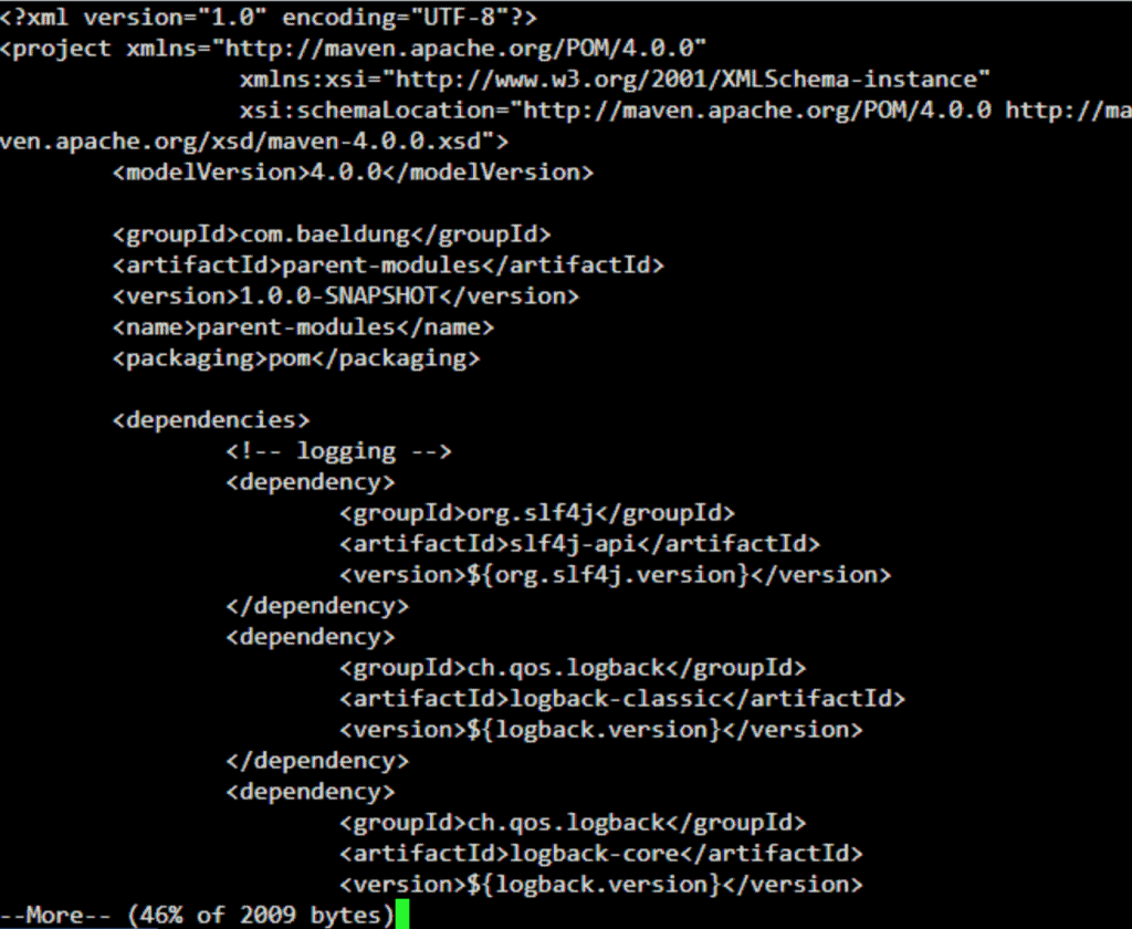
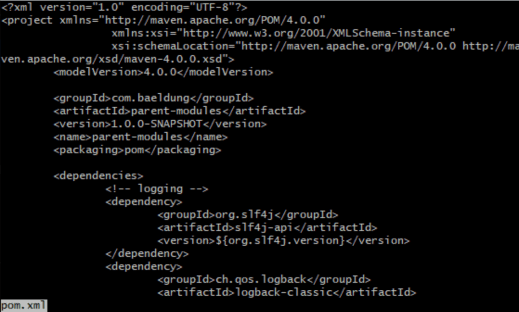
Let's explore the project layout created by Apache Tapestry:
![]()
We can see a Maven-like project structure, along with a few packages based on conventions.
The Java classes are placed in src/main/java and categorized as components, pages, and services.
Likewise, src/main/resources hold our templates (similar to HTML files) — these have the .tml extension.
For every Java class placed under components and pages directories, a template file with the same name should be created.
The src/main/webapp directory contains resources like images, stylesheets, and JavaScript files. Similarly, testing files are placed in src/test.
Last, src/site will contain the documentation files.
For a better idea, let's take a look at the project structure opened in Eclipse IDE:
![]()
5. Annotations
Let's discuss a few handy annotations provided by Apache Tapestry for day-to-day use. Going forward, we'll use these annotations in our implementations.
5.1. @Inject
The @Inject annotation is available in the org.apache.tapestry5.ioc.annotations package and provides an easy way to inject dependencies in Java classes.
This annotation is quite handy to inject an asset, block, resource, and service.
5.2. @InjectPage
Available in the org.apache.tapestry5.annotations package, the @InjectPage annotation allows us to inject a page into another component. Also, the injected page is always a read-only property.
5.3. @InjectComponent
Similarly, the @InjectComponent annotation allows us to inject a component defined in the template.
5.4. @Log
The @Log annotation is available in the org.apache.tapestry5.annotations package and is handy to enable the DEBUG level logging on any method. It logs method entry and exit, along with parameter values.
5.5. @Property
Available in the org.apache.tapestry5.annotations package, the @Property annotation marks a field as a property. At the same time, it automatically creates getters and setters for the property.
5.6. @Parameter
Similarly, the @Parameter annotation denotes that a field is a component parameter.
6. Page
So, we're all set to explore the basic features of the framework. Let's create a new Home page in our app.
First, we'll define a Java class Home in the pages directory in src/main/java:
public class Home {
}
6.1. Template
Then, we'll create a corresponding Home.tml template in the pages directory under src/main/resources.
A file with the extension .tml (Tapestry Markup Language) is similar to an HTML/XHTML file with XML markup provided by Apache Tapestry.
For instance, let's have a look at the Home.tml template:
<html xmlns:t="http://tapestry.apache.org/schema/tapestry_5_4.xsd">
    <head>
        <title>apache-tapestry Home</title>
    </head>
    <body>
        <h1>Home</h1>
    </body>
</html>
Voila! Simply by restarting the Jetty server, we can access the Home page at localhost:8080/apache-tapestry/home:
![]()
6.2. Property
Let's explore how to render a property on the Home page.
For this, we'll add a property and a getter method in the Home class:
@Property
private String appName = "apache-tapestry";

public Date getCurrentTime() {
    return new Date();
}
To render the appName property on the Home page, we can simply use ${appName}.
Similarly, we can write ${currentTime} to access the getCurrentTime method from the page.
6.3. Localization
Apache Tapestry provides integrated localization support. As per convention, a page name property file keeps the list of all the local messages to render on the page.
For instance, we'll create a home.properties file in the pages directory for the Home page with a local message:
introMsg=Welcome to the Apache Tapestry Tutorial
The message properties are different from the Java properties.
For the same reason, the key name with the message prefix is used to render a message property — for instance, ${message:introMsg}.
6.4. Layout Component
Let's define a basic layout component by creating the Layout.java class. We'll keep the file in the components directory in src/main/java:
public class Layout {
    @Property
    @Parameter(required = true, defaultPrefix = BindingConstants.LITERAL)
    private String title;
}
Here, the title property is marked required, and the default prefix for binding is set as literal String.
Then, we'll write a corresponding template file Layout.tml in the components directory in src/main/resources:
<html xmlns:t="http://tapestry.apache.org/schema/tapestry_5_4.xsd">
    <head>
        <title>${title}</title>
    </head>
    <body>
        <div class="container">
            <t:body />
            <hr/>
            <footer>
                <p>© Your Company</p>
            </footer>
        </div>
    </body>
</html>
Now, let's use the layout on the home page:
<html t:type="layout" title="apache-tapestry Home"
    xmlns:t="http://tapestry.apache.org/schema/tapestry_5_4.xsd">
    <h1>Home! ${appName}</h1>
    <h2>${message:introMsg}</h2>
    <h3>${currentTime}</h3>
</html>
Note, the namespace is used to identify the elements (t:type and t:body) provided by Apache Tapestry. At the same time, the namespace also provides components and attributes.
Here, the t:type will set the layout on the home page. And, the t:body element will insert the content of the page.
Let's take a look at the Home page with the layout:
![]()
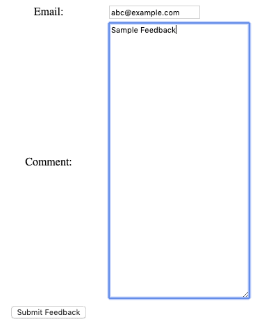
7. Form
Let's create a Login page with a form, to allow users to sign-in.
As already explored, we'll first create a Java class Login:
public class Login {
    // ...
    @InjectComponent
    private Form login;

    @Property
    private String email;

    @Property
    private String password;
}
Here, we've defined two properties — email and password. Also, we've injected a Form component for the login.
Then, let's create a corresponding template login.tml:
<html t:type="layout" title="apache-tapestry com.example"
      xmlns:t="http://tapestry.apache.org/schema/tapestry_5_3.xsd"
      xmlns:p="tapestry:parameter">
    <t:form t:id="login">
        <h2>Please sign in</h2>
        <t:textfield t:id="email" placeholder="Email address"/>
        <t:passwordfield t:id="password" placeholder="Password"/>
        <t:submit class="btn btn-large btn-primary" value="Sign in"/>
    </t:form>
</html>
Now, we can access the login page at localhost:8080/apache-tapestry/login:
![]()
8. Validation
Apache Tapestry provides a few built-in methods for form validation. It also provides ways to handle the success or failure of the form submission.
The built-in method follows the convention of the event and the component name. For instance, the method onValidationFromLogin will validate the Login component.
Likewise, methods like onSuccessFromLogin and onFailureFromLogin are for success and failure events respectively.
So, let's add these built-in methods to the Login class:
public class Login {
    // ...

    void onValidateFromLogin() {
        if (email == null)
            System.out.println("Email is null);

        if (password == null)
            System.out.println("Password is null);
    }

    Object onSuccessFromLogin() {
        System.out.println("Welcome! Login Successful");
        return Home.class;
    }

    void onFailureFromLogin() {
        System.out.println("Please try again with correct credentials");
    }
}
9. Alerts
Form validation is incomplete without proper alerts. Not to mention, the framework also has built-in support for alert messages.
For this, we'll first inject the instance of the AlertManager in the Login class to manage the alerts. Then, replace the println statements in existing methods with the alert messages:
public class Login {
    // ...
    @Inject
    private AlertManager alertManager;

    void onValidateFromLogin() {
        if(email == null || password == null) {
            alertManager.error("Email/Password is null");
            login.recordError("Validation failed"); //submission failure on the form
        }
    }

    Object onSuccessFromLogin() {
        alertManager.success("Welcome! Login Successful");
        return Home.class;
    }

    void onFailureFromLogin() {
        alertManager.error("Please try again with correct credentials");
    }
}
Let's see the alerts in action when the login fails:
![]()
10. Ajax
So far, we've explored the creation of a simple home page with a form. At the same time, we've seen the validations and support for alert messages.
Next, let's explore the Apache Tapestry's built-in support for Ajax.
First, we'll inject the instance of the AjaxResponseRenderer and Block component in the Home class. Then, we'll create a method onCallAjax for processing the Ajax call:
public class Home {
    // ....

    @Inject
    private AjaxResponseRenderer ajaxResponseRenderer;

    @Inject
    private Block ajaxBlock;

    @Log
    void onCallAjax() {
        ajaxResponseRenderer.addRender("ajaxZone", ajaxBlock);
    }
}
Also, we need to make a few changes in our Home.tml.
First, we'll add the eventLink to invoke the onCallAjax method. Then, we'll add a zone element with id ajaxZone to render the Ajax response.
Last, we need to have a block component that will be injected in the Home class and rendered as Ajax response:
<p><t:eventlink event="callAjax" zone="ajaxZone" class="btn btn-default">Call Ajax</t:eventlink></p>
<t:zone t:id="ajaxZone"></t:zone>
<t:block t:id="ajaxBlock">
    <hr/>
    <h2>Rendered through Ajax</h2>
    <p>The current time is: <strong>${currentTime}</strong></p>
</t:block>
Let's take a look at the updated home page:
![]()
Then, we can click the Call Ajax button and see the ajaxResponseRenderer in action:
![]()
11. Logging
To enable the built-in logging feature, the instance of the Logger is required to be injected. Then, we can use it to log at any level like TRACE, DEBUG, and INFO.
So, let's make the required changes in the Home class:
public class Home {
    // ...

    @Inject
    private Logger logger;

    void onCallAjax() {
        logger.info("Ajax call");
        ajaxResponseRenderer.addRender("ajaxZone", ajaxBlock);
    }
}
Now, when we click the Call Ajax button, the logger will log at the INFO level:
[INFO] pages.Home Ajax call
12. Conclusion
In this article, we've explored the Apache Tapestry web framework.
To begin with, we've created a quickstart web application and added a Home page using basic features of Apache Tapestry, like components, pages, and templates.
Then, we've examined a few handy annotations provided by Apache Tapestry to configure a property and component/page injection.
Last, we've explored the built-in Ajax and logging support provided by the framework.
As usual, all the code implementations are available over on GitHub.
![]()