1. Overview

One of the features of Java JSR 380 is allowing expressions while interpolating the validation messages with parameters.

When we use Hibernate Validator, there is a requirement that we need to add one of the uniform implementations of Java JSR 341 as a dependency to our project. JSR 341 is also called the Expression Language API.

However, adding an extra library can be cumbersome if we don't need to support parsing expressions according to our use-case.

In this short tutorial, we'll have a look at how to configure ParameterMessageInterpolator in Hibernate Validator.

2. Message Interpolators

Beyond the basics of validating a Java bean, the Bean Validation API's MessageInterpolator is an abstraction that gives us a way of performing simple interpolations without the hassle of parsing expressions.

Besides, Hibernate Validator offers a non-expression based ParameterMessageInterpolator, and therefore, we don't need any extra libraries to configure it.

3. Setting up Custom Message Interpolators

To remove the expression language dependency, we can use custom message interpolators and configure Hibernate Validator without expression support.

Let's show some of the convenient ways of setting up custom message interpolators. We'll use the built-in ParameterMessageInterpolator in our case.

3.1. Configuring ValidatorFactory

One way of setting up a custom message interpolator is to configure ValidatorFactory when bootstrapping.

Thus, we can build a ValidatorFactory instance with ParameterMessageInterpolator:

ValidatorFactory validatorFactory = Validation.byDefaultProvider()
  .configure()
  .messageInterpolator(new ParameterMessageInterpolator())
  .buildValidatorFactory();

3.2. Configuring Validator

Similarly, we can set ParameterMessageInterpolator when we initialize the Validator instance:

Validator validator = validatorFactory.usingContext()
  .messageInterpolator(new ParameterMessageInterpolator())
  .getValidator();

4. Performing Validations

To see how ParameterMessageInterpolator works, we need a sample Java bean with some JSR 380 annotations on it.

4.1. Sample Java Bean

Let's define our sample Java bean Person:

public class Person {

    @Size(min = 10, max = 100, message = "Name should be between {min} and {max} characters")
    private String name;

    @Min(value = 18, message = "Age should not be less than {value}")
    private int age;

    @Email(message = "Email address should be in a correct format: ${validatedValue}")
    private String email;

    // standard getters and setters
}

4.2. Testing Message Parameters

Certainly, to perform our validations, we should use a Validator instance accessed from ValidatorFactory, which we already configured before.

So, we need to access our Validator:

Validator validator = validatorFactory.getValidator();

After that, we can write our test method for the name field:

@Test
public void givenNameLengthLessThanMin_whenValidate_thenValidationFails() {
    Person person = new Person();
    person.setName("John Doe");
    person.setAge(18);

    Set<ConstraintViolation<Person>> violations = validator.validate(person);
 
    assertEquals(1, violations.size());

    ConstraintViolation<Person> violation = violations.iterator().next();
 
    assertEquals("Name should be between 10 and 100 characters", violation.getMessage());
}

The validation message is interpolated with variables of {min} and {max} correctly:

Name should be between 10 and 100 characters

Next, let's write a similar test for the age field:

@Test
public void givenAgeIsLessThanMin_whenValidate_thenValidationFails() {
    Person person = new Person();
    person.setName("John Stephaner Doe");
    person.setAge(16);

    Set<ConstraintViolation<Person>> violations = validator.validate(person);
 
    assertEquals(1, violations.size());

    ConstraintViolation<Person> violation = violations.iterator().next();
 
    assertEquals("Age should not be less than 18", violation.getMessage());
}

Similarly, the validation message is interpolated correctly with the variable {value} as we expected:

Age should not be less than 18

4.3. Testing Expressions

To see how ParameterMessageInterpolator behaves with expressions, let's write another test for the email field that involves a simple ${validatedValue} expression:

@Test
public void givenEmailIsMalformed_whenValidate_thenValidationFails() {
    Person person = new Person();
    person.setName("John Stephaner Doe");
    person.setAge(18);
    person.setEmail("johndoe.dev");
    
    Set<ConstraintViolation<Person>> violations = validator.validate(person);
 
    assertEquals(1, violations.size());
    
    ConstraintViolation<Person> violation = violations.iterator().next();
 
    assertEquals("Email address should be in a correct format: ${validatedValue}", violation.getMessage());
}

This time, the expression ${validatedValue} is not interpolated.

ParameterMessageInterpolator only supports the interpolation of parameters, not parsing expressions that use the $ notation. Instead, it simply returns them un-interpolated.

5. Conclusion

In this article, we learned what ParameterMessageInterpolator is for and how to configure it in Hibernate Validator.

As always, all the examples involved in this tutorial are available over on GitHub.

1. Overview

In this tutorial, we'll briefly look at the nextLine() method of java.util.Scanner class. Furthermore, we'll see an example of its usage.

2. Scanner.nextLine()

The nextLine() method of the java.util.Scanner class scans from the current position until it finds a line separator delimiter. The method returns the String from the current position to the end of the line. Consequently, after the operation, the position of the scanner is set to the beginning of the next line that follows the delimiter.

The method will search through the input data looking for a line separator. It may scan all of the input data searching for the line to skip if no line separators are present.

The signature of the nextLine() method is:

public String nextLine()

The method takes no parameters. It returns the current line, excluding any line separator at the end.

Let's look at its usage:

try (Scanner scanner = new Scanner("Scanner\nTest\n")) {
    assertEquals("Scanner", scanner.nextLine());
    assertEquals("Test", scanner.nextLine());
}

As we have seen, the method returns the input from the current scanner position until the line separator is found:

try (Scanner scanner = new Scanner("Scanner\n")) {
    scanner.useDelimiter("");
    scanner.next();
    assertEquals("canner", scanner.nextLine());
}

In the above example, the call to next() returns ‘S' and advances the scanner position to point to ‘c'. Therefore, when we call nextLine() method it returns the input from the current scanner position until it finds a line separator.

The nextLine() method throws two types of checked exceptions.

Firstly, when no line separator is found, it throws NoSuchElementException:

@Test(expected = NoSuchElementException.class)
public void whenReadingLines_thenThrowNoSuchElementException() {
    try (Scanner scanner = new Scanner("")) {
        scanner.nextLine();
    }
}

Secondly, it throws IllegalStateException if the scanner is closed:

@Test(expected = IllegalStateException.class)
public void whenReadingLines_thenThrowIllegalStateException() {
    Scanner scanner = new Scanner("");
    scanner.close();
    scanner.nextLine();
}

3. Conclusion

In this quick article, we looked at the nextLine() method of Java's Scanner class. Furthermore, we looked at its usage in a simple Java program. Finally, we looked at the exceptions that are thrown by the method and sample code illustrating it.

As always, the full source code of the working examples is available over on GitHub.

1. Introduction

When working with Hibernate, we can use named parameters to safely pass data into an SQL query. We assign values to query parameters at runtime to make them dynamic. More importantly, this helps prevent SQL injection attacks.

However, we may encounter errors when working with named parameters. Two of the more common ones from Hibernate's standalone library and the Hibernate JPA implementation, respectively, are:

• Not all named parameters have been set
• Named parameter not bound

Although the error messages may differ between vanilla Hibernate and its JPA implementation, the root cause is the same.

In this tutorial, we'll take a look at what causes these errors and how to avoid them. Along the way, we'll demonstrate how to use named parameters with Hibernate's standalone library.

2. What Causes the Error

When working with named parameters in Hibernate, we must assign a value to each named parameter before executing the query.

Let's look at an example of a query that uses a named parameter:

Query<Event> query = session.createQuery("from Event E WHERE E.title = :eventTitle", Event.class);

In this example, we have one named parameter, indicated by the :eventTitle placeholder. Hibernate expects this parameter to be set before we execute the query.

However, if we try to execute the query without setting the value for :eventTitle:

List<Event> listOfEvents = query.list();

Hibernate will throw org.hibernate.QueryException when we run it, and we'll get the error:

Not all named parameters have been set

3. Fixing the Error

To fix the error, we simply provide a value for the named parameter before executing the query:

Query<Event> query = session.createQuery("from Event E WHERE E.title = :eventTitle", Event.class);
query.setParameter("eventTitle", "Event 1");
 
assertEquals(1, query.list().size());

By using the setParameter(String, String) method of the query object, we tell Hibernate which value we want to use for the named parameter.

4. Conclusion

In this article, we looked at named parameters and how they are used in Hibernate. We also showed how to fix one of the named query errors we might run into.

As usual, all the code samples are available over on GitHub.

1. Overview

Session per request is a transactional pattern to tie the persistence session and request life-cycles together. Not surprisingly, Spring comes with its own implementation of this pattern, named OpenSessionInViewInterceptor, to facilitate working with lazy associations and therefore, improving developer productivity.

In this tutorial, first, we're going to learn how the interceptor works internally, and then, we'll see how this controversial pattern can be a double-edged sword for our applications!

2. Introducing Open Session in View

To better understand the role of Open Session in View (OSIV), let's suppose we have an incoming request:

1. Spring opens a new Hibernate Session at the beginning of the request. These Sessions are not necessarily connected to the database.
2. Every time the application needs a Session, it will reuse the already existing one.
3. At the end of the request, the same interceptor closes that Session.

At first glance, it might make sense to enable this feature. After all, the framework handles the session creation and termination, so the developers don't concern themselves with these seemingly low-level details. This, in turn, boosts developer productivity.

However, sometimes, OSIV can cause subtle performance issues in production. Usually, these types of issues are very hard to diagnose.

2.1. Spring Boot

By default, OSIV is active in Spring Boot applications. Despite that, as of Spring Boot 2.0, it warns us of the fact that it's enabled at application startup if we haven't configured it explicitly:

spring.jpa.open-in-view is enabled by default. Therefore, database 
queries may be performed during view rendering.Explicitly configure 
spring.jpa.open-in-view to disable this warning

Anyway, we can disable the OSIV by using the spring.jpa.open-in-view configuration property:

spring.jpa.open-in-view=false

2.2. Pattern or Anti-Pattern?

There have always been mixed reactions towards OSIV. The main argument of the pro-OSIV camp is developer productivity, especially when dealing with lazy associations.

On the other hand, database performance issues are the primary argument of the anti-OSIV campaign. Later on, we're going to assess both arguments in detail.

3. Lazy Initialization Hero

Since OSIV binds the Session lifecycle to each request, Hibernate can resolve lazy associations even after returning from an explicit @Transactional service.

To better understand this, let's suppose we're modeling our users and their security permissions:

@Entity
@Table(name = "users")
public class User {

    @Id
    @GeneratedValue
    private Long id;

    private String username;

    @ElementCollection
    private Set<String> permissions;

    // getters and setters
}

Similar to other one-to-many and many-to-many relationships, the permissions property is a lazy collection.

Then, in our service layer implementation, let's explicitly demarcate our transactional boundary using @Transactional:

@Service
public class SimpleUserService implements UserService {

    private final UserRepository userRepository;

    public SimpleUserService(UserRepository userRepository) {
        this.userRepository = userRepository;
    }

    @Override
    @Transactional(readOnly = true)
    public Optional<User> findOne(String username) {
        return userRepository.findByUsername(username);
    }
}

3.1. The Expectation

Here's what we expect to happen when our code calls the findOne method:

1. At first, the Spring proxy intercepts the call and gets the current transaction or creates one if none exists.
2. Then, it delegates the method call to our implementation.
3. Finally, the proxy commits the transaction and consequently closes the underlying Session. After all, we only need that Session in our service layer.

In the findOne method implementation, we didn't initialize the permissions collection. Therefore, we shouldn't be able to use the permissions after the method returns. If we do iterate on this property, we should get a LazyInitializationException.

3.2. Welcome to the Real World

Let's write a simple REST controller to see if we can use the permissions property:

@RestController
@RequestMapping("/users")
public class UserController {

    private final UserService userService;

    public UserController(UserService userService) {
        this.userService = userService;
    }

    @GetMapping("/{username}")
    public ResponseEntity<?> findOne(@PathVariable String username) {
        return userService
                .findOne(username)
                .map(DetailedUserDto::fromEntity)
                .map(ResponseEntity::ok)
                .orElse(ResponseEntity.notFound().build());
    }
}

Here, we iterate over permissions during entity to DTO conversion. Since we expect that conversion to fail with a LazyInitializationException, the following test shouldn't pass:

@SpringBootTest
@AutoConfigureMockMvc
@ActiveProfiles("test")
class UserControllerIntegrationTest {

    @Autowired
    private UserRepository userRepository;

    @Autowired
    private MockMvc mockMvc;

    @BeforeEach
    void setUp() {
        User user = new User();
        user.setUsername("root");
        user.setPermissions(new HashSet<>(Arrays.asList("PERM_READ", "PERM_WRITE")));

        userRepository.save(user);
    }

    @Test
    void givenTheUserExists_WhenOsivIsEnabled_ThenLazyInitWorksEverywhere() throws Exception {
        mockMvc.perform(get("/users/root"))
          .andExpect(status().isOk())
          .andExpect(jsonPath("$.username").value("root"))
          .andExpect(jsonPath("$.permissions", containsInAnyOrder("PERM_READ", "PERM_WRITE")));
    }
}

However, this test doesn't throw any exceptions, and it passes.

Because OSIV creates a Session at the beginning of the request, the transactional proxy uses the current available Session instead of creating a brand new one.

So, despite what we might expect, we actually can use the permissions property even outside of an explicit @Transactional. Moreover, these sorts of lazy associations can be fetched anywhere in the current request scope.

3.3. On Developer Productivity

If OSIV wasn't enabled, we'd have to manually initialize all necessary lazy associations in a transactional context. The most rudimentary (and usually wrong) way is to use the Hibernate.initialize() method:

@Override
@Transactional(readOnly = true)
public Optional<User> findOne(String username) {
    Optional<User> user = userRepository.findByUsername(username);
    user.ifPresent(u -> Hibernate.initialize(u.getPermissions()));

    return user;
}

By now, the effect of OSIV on developer productivity is obvious. However, it's not always about developer productivity.

4. Performance Villain

Suppose we have to extend our simple user service to call another remote service after fetching the user from the database:

@Override
public Optional<User> findOne(String username) {
    Optional<User> user = userRepository.findByUsername(username);
    if (user.isPresent()) {
        // remote call
    }

    return user;
}

Here, we're removing the @Transactional annotation since we clearly won't want to keep the connected Session while waiting for the remote service.

4.1. Avoiding Mixed IOs

Let's clarify what happens if we don't remove the @Transactional annotation. Suppose the new remote service is responding a little more slowly than usual:

1. At first, the Spring proxy gets the current Session or creates a new one. Either way, this Session is not connected yet. That is, it's not using any connection from the pool.
2. Once we execute the query to find a user, the Session becomes connected and borrows a Connection from the pool.
3. If the whole method is transactional, then the method proceeds to call the slow remote service while keeping the borrowed Connection.

Imagine that during this period, we get a burst of calls to the findOne method. Then, after a while, all Connections may wait for a response from that API call. Therefore, we may soon run out of database connections.

Mixing database IOs with other types of IOs in a transactional context is a bad smell, and we should avoid it at all costs.

Anyway, since we removed the @Transactional annotation from our service, we're expecting to be safe.

4.2. Exhausting the Connection Pool

When OSIV is active, there is always a Session in the current request scope, even if we remove @Transactional. Although this Session is not connected initially, after our first database IO, it gets connected and remains so until the end of the request.

So, our innocent-looking and recently-optimized service implementation is a recipe for disaster in the presence of OSIV:

@Override
public Optional<User> findOne(String username) {
    Optional<User> user = userRepository.findByUsername(username);
    if (user.isPresent()) {
        // remote call
    }

    return user;
}

Here's what happens while the OSIV is enabled:

1. At the beginning of the request, the corresponding filter creates a new Session.
2. When we call the findByUsername method, that Session borrows a Connection from the pool.
3. The Session remains connected until the end of the request.

Even though we're expecting that our service code won't exhaust the connection pool, the mere presence of OSIV can potentially make the whole application unresponsive.

To make matters even worse, the root cause of the problem (slow remote service) and the symptom (database connection pool) are unrelated. Because of this little correlation, such performance issues are difficult to diagnose in production environments.

4.3. Unnecessary Queries

Unfortunately, exhausting the connection pool is not the only OSIV-related performance issue.

Since the Session is open for the entire request lifecycle, some property navigations may trigger a few more unwanted queries outside of the transactional context. It's even possible to end up with n+1 select problem, and the worst news is that we may not notice this until production.

Adding insult to injury, the Session executes all those extra queries in auto-commit mode. In auto-commit mode, each SQL statement is treated as a transaction and is automatically committed right after it is executed. This, in turn, puts a lot of pressure on the database.

5. Choose Wisely

Whether the OSIV is a pattern or an anti-pattern is irrelevant. The most important thing here is the reality in which we're living.

If we're developing a simple CRUD service, it might make sense to use the OSIV, as we may never encounter those performance issues.

On the other hand, if we find ourselves calling a lot of remote services or there is so much going on outside of our transactional contexts, it's highly recommended to disable the OSIV altogether. 

When in doubt, start without OSIV, since we can easily enable it later. On the other hand, disabling an already enabled OSIV may be cumbersome, as we may need to handle a lot of LazyInitializationExceptions.

The bottom line is that we should be aware of the trade-offs when using or ignoring the OSIV.

6. Alternatives

If we disable OSIV, then we should somehow prevent potential LazyInitializationExceptions when dealing with lazy associations. Among a handful of approaches to coping with lazy associations, we're going to enumerate two of them here.

6.1. Entity Graphs

When defining query methods in Spring Data JPA, we can annotate a query method with @EntityGraph to eagerly fetch some part of the entity:

public interface UserRepository extends JpaRepository<User, Long> {

    @EntityGraph(attributePaths = "permissions")
    Optional<User> findByUsername(String username);
}

Here, we're defining an ad-hoc entity graph to load the permissions attribute eagerly, even though it's a lazy collection by default.

If we need to return multiple projections from the same query, then we should define multiple queries with different entity graph configurations:

public interface UserRepository extends JpaRepository<User, Long> {
    @EntityGraph(attributePaths = "permissions")
    Optional<User> findDetailedByUsername(String username);

    Optional<User> findSummaryByUsername(String username);
}

6.2. Caveats When Using Hibernate.initialize()

One might argue that instead of using entity graphs, we can use the notorious Hibernate.initialize() to fetch lazy associations wherever we need to do so:

@Override
@Transactional(readOnly = true)
public Optional<User> findOne(String username) {
    Optional<User> user = userRepository.findByUsername(username);
    user.ifPresent(u -> Hibernate.initialize(u.getPermissions()));
        
    return user;
}

They may be clever about it and also suggest to call the getPermissions() method to trigger the fetching process:

Optional<User> user = userRepository.findByUsername(username);
user.ifPresent(u -> {
    Set<String> permissions = u.getPermissions();
    System.out.println("Permissions loaded: " + permissions.size());
});

Both approaches aren't recommended since they incur (at least) one extra query, in addition to the original one, to fetch the lazy association. That is, Hibernate generates the following queries to fetch users and their permissions:

> select u.id, u.username from users u where u.username=?
> select p.user_id, p.permissions from user_permissions p where p.user_id=?

Although most databases are pretty good at executing the second query, we should avoid that extra network round-trip.

On the other hand, if we use entity graphs or even Fetch Joins, Hibernate would fetch all the necessary data with just one query:

> select u.id, u.username, p.user_id, p.permissions from users u 
  left outer join user_permissions p on u.id=p.user_id where u.username=?

7. Conclusion

In this article, we turned our attention towards a pretty controversial feature in Spring and a few other enterprise frameworks: Open Session in View. First, we got aquatinted with this pattern both conceptually and implementation-wise. Then we analyzed it from productivity and performance perspectives.

As usual, the sample code is available over on GitHub.

1. Introduction

In this tutorial, we'll learn how to read the body from the HttpServletRequest multiple times using Spring.

HttpServletRequest is an interface which exposes getInputStream()  method to read the body. By default, the data from this InputStream can be read only once.

2. Maven Dependencies

The first thing we'll need is the appropriate spring-webmvc and javax.servlet dependencies:

<dependency>
    <groupId>org.springframework</groupId>
    <artifactId>spring-webmvc</artifactId>
    <version>5.2.0.RELEASE</version>
</dependency>
<dependency>
    <groupId>javax.servlet</groupId>
    <artifactId>javax.servlet-api</artifactId>
    <version>4.0.1</version>
</dependency>

Also, since we're using the application/json content-type, the jackson-databind dependency is required:

<dependency>
    <groupId>com.fasterxml.jackson.core</groupId>
    <artifactId>jackson-databind</artifactId>
    <version>2.10.0</version>
</dependency>

Spring uses this library to convert to and from JSON.

3. Spring's ContentCachingRequestWrapper

Spring provides a ContentCachingRequestWrapper class. This class provides a method, getContentAsByteArray() to read the body multiple times.

This class has a limitation, though:  We can't read the body multiple times using the getInputStream() and getReader() methods.

This class caches the request body by consuming the InputStream. If we read the InputStream in one of the filters, then other subsequent filters in the filter chain can't read it anymore. Because of this limitation, this class is not suitable in all situations.

To overcome this limitation, let's now take a look at a more general-purpose solution.

4. Extending HttpServletRequest

Let's create a new class – CachedBodyHttpServletRequest – which extends HttpServletRequestWrapper. This way, we don't need to override all the abstract methods of the HttpServletRequest interface.

HttpServletRequestWrapper class has two abstract methods getInputStream() and getReader(). We'll override both of these methods and create a new constructor.

4.1. The Constructor

First, let's create a constructor. Inside it, we'll read the body from the actual InputStream and store it in a byte[] object:

public class CachedBodyHttpServletRequest extends HttpServletRequestWrapper {

    private byte[] cachedBody;

    public CachedBodyHttpServletRequest(HttpServletRequest request) throws IOException {
        super(request);
        InputStream requestInputStream = request.getInputStream();
        this.cachedBody = StreamUtils.copyToByteArray(requestInputStream);
    }
}

As a result, we'll be able to read the body multiple times.

4.2. getInputStream()

Next, let's override the getInputStream() method. We'll use this method to read the raw body and convert it into an object.

In this method, we'll create and return a new object of CachedBodyServletInputStream class (an implementation of ServletInputStream):

@Override
public ServletInputStream getInputStream() throws IOException {
    return new CachedBodyServletInputStream(this.cachedBody);
}

4.3. getReader()

Then, we'll override the getReader() method. This method returns a BufferedReader object:

@Override
public BufferedReader getReader() throws IOException {
    ByteArrayInputStream byteArrayInputStream = new ByteArrayInputStream(this.cachedBody);
    return new BufferedReader(new InputStreamReader(byteArrayInputStream));
}

5. Implementation of ServletInputStream

Let's create a class – CachedBodyServletInputStream – which will implement ServletInputStream. In this class, we'll create a new constructor as well as override the isFinished(), isReady() and read() methods.

5.1. The Constructor

First, let's create a new constructor that takes a byte array.

Inside it, we'll create a new ByteArrayInputStream instance using that byte array. After that, we'll assign it to the global variable cachedBodyInputStream:

public class CachedBodyServletInputStream extends ServletInputStream {

    private InputStream cachedBodyInputStream;

    public CachedBodyServletInputStream(byte[] cachedBody) {
        this.cachedBodyInputStream = new ByteArrayInputStream(cachedBody);
    }
}

5.2. read()

Then, we'll override the read() method. In this method, we'll call ByteArrayInputStream#read:

@Override
public int read() throws IOException {
    return cachedBodyInputStream.read();
}

5.3. isFinished()

Then, we'll override the isFinished() method. This method indicates whether InputStream has more data to read or not. It returns true when zero bytes available to read:

@Override
public boolean isFinished() {
    return cachedBody.available() == 0;
}

5.4. isReady()

Similarly, we'll override the isReady() method. This method indicates whether InputStream is ready for reading or not.

Since we've already copied InputStream in a byte array, we'll return true to indicate that it's always available:

@Override
public boolean isReady() {
    return true;
}

6. The Filter

Finally, let's create a new filter to make use of the CachedBodyHttpServletRequest class. Here we'll extend Spring's OncePerRequestFilter class. This class has an abstract method doFilterInternal().

In this method, we'll create an object of the CachedBodyHttpServletRequest class from the actual request object:

CachedBodyHttpServletRequest cachedBodyHttpServletRequest =
  new CachedBodyHttpServletRequest(request);

Then we'll pass this new request wrapper object to the filter chain. So, all the subsequent calls to the getInputStream() method will invoke the overridden method:

filterChain.doFilter(cachedContentHttpServletRequest, response);

7. Conclusion

In this tutorial, we quickly walked through the ContentCachingRequestWrapper class. We also saw its limitations.

Then, we created a new implementation of the HttpServletRequestWrapper class. We overrode the getInputStream() method to return an object of ServletInputStream class.

Finally, we created a new filter to pass the request wrapper object to the filter chain. So, we were able to read the request multiple times.

The full source code of the examples can be found over on GitHub.

1. Introduction

In this tutorial, we'll introduce the Unix swap space, its advantages, and a few simple commands to manage it.

2. The Unix Swap Space

Swap or paging space is basically a portion of the hard disk that the operating system can use as an extension of the available RAM. This space can be allocated with a partition or a simple file.

Thanks to a memory paging technique, specifically the virtual memory management technique, our OS is able to load applications that require more memory than the RAM physically present in our computer.

When the RAM is full, portions of active applications' data are transferred to the swap space, freeing up RAM for other data needed immediately.

The reasons behind the implementation of this technique are historical: the first machine to feature virtual memory was the Atlas super-computer built in Cambridge in the 1960s, when physical memory was very expensive.

The savings, the additional security, and the increased reliability provided a strong incentive to switch all systems to virtual memory.

3. Create a Swap Space

As mentioned earlier, the swap is a space reserved for memory management.

We have two ways to tell the OS where this space is to be allocated. We can create a new file within an existing partition, or we can allocate an entire partition of type swap.

3.1. Create a Swap File

First of all, we need to create an empty file with the desired size.

To do that, we use the dd command, configuring the size options appropriately:

• bs – controls the number of bytes to write in one go as a block
• count – refers to the number of blocks to write

Let's create a 4 GB swap file with 4,096 blocks, at 1 MB per block:

sudo dd if=/dev/zero of=/myswapfile bs=1M count=4096

# Output
4096+0 records in
4096+0 records out
4294967296 bytes (4.3 GB, 4.0 GiB) copied, 20.0082 s, 215 MB/s

Now, let's set the correct permissions with chmod:

sudo chmod 600 /myswapfile

The next step is to set the file as swap space using the command mkswap:

sudo mkswap /myswapfile

# Output
Setting up swapspace version 1, size = 4 GiB (4294963200 bytes)
no label, UUID=20721910-090f-4c2a-8442-0e6f50c9c1d6

and enable it with swapon:

sudo swapon /myswapfile

Finally, we'll make our changes permanent by modifying the fstab file, in case we need to restart the machine.

To append the configuration at the end of the file we echo it to the standard output and pipe it into tee, which can parse the input line by line:

echo "/myswapfile swap swap defaults 0 0" | sudo tee -a /etc/fstab

3.2. Create a Swap Partition

The partition case is different from the previous case only because of the format used — instead of a file, we can allocate an entire portion of the disk.

In order to do that, we need to modify the partitions table to make space and create a new partition of type swap.

There are plenty of GUI tools (such as GParted) that can easily change the partitions table securely and visually with just a few mouse clicks.

Once the new partition is saved, let's define it as swap:

mkswap /dev/sdXX

mkswap: /dev/sdXX: warning: wiping old swap signature.
Setting up swapspace version 1, size = 4.0 GiB (5266130944‬ bytes)
no label, UUID=a0a2d61c-bc3a-442a-acf1-120ecb041f9d

Where sdXX should be replaced with the new partition name.

Then, we activate it:

sudo swapon /dev/sdXX

Finally, like in the file scenario, we have to add the new partition to our fstab file, so that it loads the next time we restart:

echo "/dev/sdXX swap swap defaults 0 0" | sudo tee -a /etc/fstab

4. Monitor the Swap Space

Now that our swap space is active, we may need to monitor how the OS is using it. To do this, we have various commands available that can give us information about the free swap left, some more graphical than others.

Let's explore a few simple examples of text-based solutions.

4.1. swapon –show

The swapon command usually activates a swap space, but if we specify the –show option, it will return data about the active swap spaces:

sudo swapon --show

# Output
NAME         TYPE       SIZE USED PRIO
/myswapfile  file       4024M   0B   -2
/dev/sdXX    partition  4G      0B   -3

4.2. free -h

The free command displays the amount of free and used memory in the system, including the swap space:

free -h

# Output
              total        used        free      shared  buff/cache   available
Mem:          4.9Gi       2.2Gi       193Mi        13Mi       2.6Gi       2.7Gi
Swap:         8.0Gi       2.0Mi       8.0Gi

4.3. cat /proc/swaps

The Unix proc filesystem contains information about various kernel data structures, including swap:

cat /proc/swaps

# Output
Filename				Type		Size	Used	Priority
/myswapfile                             file		4194300	2272	-2
/dev/sdXX                               partition	4194300 0	-3

4.4. top

Often used to monitor processes and resources, top has a useful header with all kind of statistics, including those about swap:

top

# Output
top - 17:40:08 up 54 min,  1 user,  load average: 0.29, 0.22, 0.12
Tasks: 188 total,   1 running, 187 sleeping,   0 stopped,   0 zombie
%Cpu(s): 17.5 us,  0.7 sy,  0.0 ni, 81.6 id,  0.0 wa,  0.0 hi,  0.2 si,  0.0 st
MiB Mem :   5050.7 total,    840.9 free,   1555.4 used,   2654.3 buff/cache
MiB Swap:   8192.0 total,   8189.8 free,      2.2 used.   3407.1 avail Mem

5. Delete a Swap Space

In order to remove a swap space, we have to follow a few simple steps:

1. Deactivate the space to remove with swapoff:

   sudo swapoff /myswapfile

2. Remove the swap entry from /etc/fstab
3. Remove the file or partition

That's all we need to reset the machine to its original state.

6. Conclusion

In this tutorial, we explored briefly what the Unix swap space is used for and how to manage it using a few simple shell commands.

1. Spring and Java

>> Azure Spring Cloud Is Now In Public Preview [spring.io]

A quick look at the Azure runtime platform for Spring Boot and Spring Cloud, developed jointly by Microsoft and Pivotal. Very cool!

>> Java Feature Spotlight: Local Variable Type Inference [infoq.com]

Making the most of this feature requires a good understanding of Java's type system.

>> Building Microservices with Spring Boot – Part 1 [blog.scottlogic.com]

And a new series on microservices begins with a basic hands-on guide using Spring Boot, Spring Cloud, and Netflix OSS.

Also worth reading:

• >> Java At Microsoft: From OpenJDK to Azure Spring Cloud [devblogs.microsoft.com]

• >> Java Heap Sizing in a Container: Quickly and Easily [blogs.oracle.com] and >> Java in a Container: Resource Allocation Guidelines [ccampo.me]

• >> Six More JEPs Proposed for JDK 14 [marxsoftware.com]

• >> Java switch – 4 wrongs don't make a right [blog.joda.org]

• >> Spring Cloud Stream – Event Routing [spring.io] and >> Spring Cloud Stream – Composed Functions or EIP [spring.io]

• >> Hibernate Tip: Best Way To Work with Scalar Projections [thoughts-on-java.org]

• >> Top 3 Maven Plugins to ensure Quality and Security for your project [rieckpil.de]

• >> Hexagonal Architecture with Java and Spring [reflectoring.io]

• >> Kotlin operators [blog.frankel.ch]

Webinars and presentations:

• >> A Bootiful Podcast: Hibernate guru Vlad Mihalcea [spring.io]

• >> Are Teams the Main Problem when Adopting LeSS? [infoq.com]

Time to upgrade:

• >> Spring Framework 5.2.1 and 5.1.11 available now [spring.io]

• >> Spring Security 5.2.1 and 5.1.7 Released [spring.io]

• >> Spring Data Moore SR1 and Lovelace SR12 released. [spring.io]

2. Technical and Musings

>> Restoring Cassandra Priam Backup with sstableloader [techblog.bozho.net]

A handy utility for selectively restoring part of a Priam-generated Cassandra backup, complete with a simple Python script for handling Snappy decompression!

>> GraphQL Search Indexing [medium.com]

And a cool use-case shows how Netflix leveraged GraphQL with Kafka and Elasticsearch to build an index for searching across data from multiple loosely-coupled services.

Also worth reading:

• >> What They Thought of Programmers. [blog.cleancoder.com]

3. Comics

And my favorite Dilberts of the week:

>> Dogbert's Sensitivity Training [dilbert.com]

>> Goofy Words [dilbert.com]

>> Dark Matter Identified [dilbert.com]

4. Pick of the Week

>> It is perfectly OK to only code at work, you can have a life too [zeroequalsfalse.com]

1. Overview

In this tutorial, we'll learn how to use JCommander to parse command-line parameters. We'll explore several of its features as we build a simple command-line application.

2. Why JCommander?

“Because life is too short to parse command line parameters” – Cédric Beust

JCommander, created by Cédric Beust, is an annotation-based library for parsing command-line parameters. It can reduce the effort of building command-line applications and help us provide a good user experience for them.

With JCommander, we can offload tricky tasks such as parsing, validation, and type conversions, to allow us to focus on our application logic.

3. Setting up JCommander

3.1. Maven Configuration

Let's begin by adding the jcommander dependency in our pom.xml:

<dependency>
    <groupId>com.beust</groupId>
    <artifactId>jcommander</artifactId>
    <version>1.78</version>
</dependency>

3.2. Hello World

Let's create a simple HelloWorldApp that takes a single input called name and prints a greeting, “Hello <name>”.

Since JCommander binds command-line arguments to fields in a Java class, we'll first define a HelloWorldArgs class with a field name annotated with @Parameter:

class HelloWorldArgs {

    @Parameter(
      names = "--name",
      description = "User name",
      required = true
    )
    private String name;
}

Now, let's use the JCommander class to parse the command-line arguments and assign the fields in our HelloWorldArgs object:

JCommander helloCmd = JCommander.newBuilder()
  .addObject(new HelloWorldArgs())
  .build();
helloCmd.parse(args);
System.out.println("Hello " + jArgs.getName());

Finally, let's invoke the main class with the same arguments from the console:

$ java HelloWorldApp --name JavaWorld
Hello JavaWorld

4. Building a Real Application in JCommander

Now that we're up and running, let's consider a more complex use case — a command-line API client that interacts with a billing application such as Stripe, particularly the Metered (or usage-based) Billing scenario. This third-party billing service manages our subscriptions and invoicing.

Let's imagine that we're running a SaaS business, in which our customers buy subscriptions to our services and are billed for the number of API calls to our services per month. We'll perform two operations in our client:

• submit: Submit quantity and unit price of usage for a customer against a given subscription
• fetch: Fetch charges for a customer based on the consumption on some or all of their subscriptions in the current month — we can get these charges aggregated over all the subscriptions or itemized by each subscription

We'll build the API client as we go through the library's features.

Let's begin!

5. Defining a Parameter

Let's begin by defining the parameters that our application can use.

5.1. The @Parameter Annotation

Annotating a field with @Parameter tells JCommander to bind a matching command-line argument to it. @Parameter has attributes to describe the main parameter, such as:

• names – one or more names of the option, for example “–name” or “-n”
• description – the meaning behind the option, to help the end user
• required – whether the option is mandatory, defaults to false
• arity – number of additional parameters that the option consumes

Let's configure a parameter customerId in our metered-billing scenario:

@Parameter(
  names = { "--customer", "-C" },
  description = "Id of the Customer who's using the services",
  arity = 1,
  required = true
)
String customerId;

Now, let's execute our command with the new “–customer” parameter:

$ java App --customer cust0000001A
Read CustomerId: cust0000001A.

Likewise, we can use the shorter “-C” parameter to achieve the same effect:

$ java App -C cust0000001A
Read CustomerId: cust0000001A.

5.2. Required Parameters

Where a parameter is mandatory, the application exits throwing a ParameterException if the user does not specify it:

$ java App
Exception in thread "main" com.beust.jcommander.ParameterException:
  The following option is required: [--customer | -C]

We should note that, in general, any error in parsing the parameters results in a ParameterException in JCommander.

6. Built-In Types

6.1. IStringConverter Interface

JCommander performs type conversion from the command-line String input into the Java types in our parameter classes. The IStringConverter interface handles type conversion of a parameter from String to any arbitrary type. So, all of JCommander's built-in converters implement this interface.

Out of the box, JCommander comes with support for common data types such as String, Integer, Boolean, BigDecimal, and Enum.

6.2. Single-Arity Types

Arity relates to the number of additional parameters an option consumes. JCommander's built-in parameter types have a default arity of one, except for Boolean and List. Therefore, common types such as  String, Integer, BigDecimal, Long, and Enum, are single-arity types.

6.3. Boolean Type

Fields of type boolean or Boolean don't need any additional parameter – these options have an arity of zero.

Let's look at an example. Perhaps we want to fetch the charges for a customer, itemized by subscription. We can add a boolean field itemized, which is false by default:

@Parameter(
  names = { "--itemized" }
)
private boolean itemized;

Our application would return aggregated charges with itemized set to false. When we invoke the command line with the itemized parameter, we set the field to true:

$ java App --itemized
Read flag itemized: true.

This works well unless we have a use case where we always want itemized charges, unless specified otherwise. We could change the parameter to be notItemized, but it might be clearer to be able to provide false as the value of itemized.

Let's introduce this behavior by using a default value true for the field, and setting its arity as one:

@Parameter(
  names = { "--itemized" },
  arity = 1
)
private boolean itemized = true;

Now, when we specify the option, the value will be set to false:

$ java App --itemized false
Read flag itemized: false.

7. List Types

JCommander provides a few ways of binding arguments to List fields.

7.1. Specifying the Parameter Multiple Times

Let's assume we want to fetch the charges of only a subset of a customer's subscriptions:

@Parameter(
  names = { "--subscription", "-S" }
)
private List<String> subscriptionIds;

The field is not mandatory, and the application would fetch the charges across all the subscriptions if the parameter is not supplied. However, we can specify multiple subscriptions by using the parameter name multiple times:

$ java App -S subscriptionA001 -S subscriptionA002 -S subscriptionA003
Read Subscriptions: [subscriptionA001, subscriptionA002, subscriptionA003].

7.2. Binding Lists using the Splitter

Instead of specifying the option multiple times, let's try to bind the list by passing a comma-separated String:

$ java App -S subscriptionA001,subscriptionA002,subscriptionA003
Read Subscriptions: [subscriptionA001, subscriptionA002, subscriptionA003].

This uses a single parameter value (arity = 1) to represent a list. JCommander will use the class CommaParameterSplitter to bind the comma-separated String to our List.

7.3. Binding Lists using a Custom Splitter

We can override the default splitter by implementing the IParameterSplitter interface:

class ColonParameterSplitter implements IParameterSplitter {

    @Override
    public List split(String value) {
        return asList(value.split(":"));
    }
}

And then mapping the implementation to the splitter attribute in @Parameter:

@Parameter(
  names = { "--subscription", "-S" },
  splitter = ColonParameterSplitter.class
)
private List<String> subscriptionIds;

Let's try it out:

$ java App -S "subscriptionA001:subscriptionA002:subscriptionA003"
Read Subscriptions: [subscriptionA001, subscriptionA002, subscriptionA003].

7.4. Variable Arity Lists

Variable arity allows us to declare lists that can take indefinite parameters, up to the next option. We can set the attribute variableArity as true to specify this behavior.

Let's try this to parse subscriptions:

@Parameter(
  names = { "--subscription", "-S" },
  variableArity = true
)
private List<String> subscriptionIds;

And when we run our command:

$ java App -S subscriptionA001 subscriptionA002 subscriptionA003 --itemized
Read Subscriptions: [subscriptionA001, subscriptionA002, subscriptionA003].

JCommander binds all input arguments following the option “-S” to the list field, until the next option or the end of the command.

7.5. Fixed Arity Lists

So far we've seen unbounded lists, where we can pass as many list items as we wish. Sometimes, we may want to limit the number of items passed to a List field. To do this, we can specify an integer arity value for a List field to make it bounded:

@Parameter(
  names = { "--subscription", "-S" },
  arity = 2
)
private List<String> subscriptionIds;

Fixed arity forces a check on the number of parameters passed to a List option and throws a ParameterException in case of a violation:

$ java App -S subscriptionA001 subscriptionA002 subscriptionA003
Was passed main parameter 'subscriptionA003' but no main parameter was defined in your arg class

The error message suggests that since JCommander expected only two arguments, it tried to parse the extra input parameter “subscriptionA003” as the next option.

8. Custom Types

We can also bind parameters by writing custom converters. Like built-in converters, custom converters must implement the IStringConverter interface.

Let's write a converter for parsing an ISO8601 timestamp:

class ISO8601TimestampConverter implements IStringConverter<Instant> {

    private static final DateTimeFormatter TS_FORMATTER = 
      DateTimeFormatter.ofPattern("uuuu-MM-dd'T'HH:mm:ss");

    @Override
    public Instant convert(String value) {
        try {
            return LocalDateTime
              .parse(value, TS_FORMATTER)
              .atOffset(ZoneOffset.UTC)
              .toInstant();
        } catch (DateTimeParseException e) {
            throw new ParameterException("Invalid timestamp");
        }
    }
}

This code will parse the input String and return an Instant, throwing a ParameterException if there's a conversion error. We can use this converter by binding it to a field of type Instant using the converter attribute in @Parameter:

@Parameter(
  names = { "--timestamp" },
  converter = ISO8601TimestampConverter.class
)
private Instant timestamp;

Let's see it in action:

$ java App --timestamp 2019-10-03T10:58:00
Read timestamp: 2019-10-03T10:58:00Z.

9. Validating Parameters

JCommander provides a few default validations:

• whether required parameters are supplied
• if the number of parameters specified matches the arity of a field
• whether each String parameter can be converted into the corresponding field's type

In addition, we may wish to add custom validations. For instance, let's assume that the customer IDs must be UUIDs.

We can write a validator for the customer field that implements the interface IParameterValidator:

class UUIDValidator implements IParameterValidator {

    private static final String UUID_REGEX = 
      "[0-9a-fA-F]{8}(-[0-9a-fA-F]{4}){3}-[0-9a-fA-F]{12}";

    @Override
    public void validate(String name, String value) throws ParameterException {
        if (!isValidUUID(value)) {
            throw new ParameterException(
              "String parameter " + value + " is not a valid UUID.");
        }
    }

    private boolean isValidUUID(String value) {
        return Pattern.compile(UUID_REGEX)
          .matcher(value)
          .matches();
    }
}

Then, we can hook it up with the validateWith attribute of the parameter:

@Parameter(
  names = { "--customer", "-C" },
  validateWith = UUIDValidator.class
)
private String customerId;

If we invoke the command with a non-UUID customer Id, the application exits with a validation failure message:

$ java App --C customer001
String parameter customer001 is not a valid UUID.

10. Sub-Commands

Now that we've learned about parameter binding, let's pull everything together to build our commands.

In JCommander, we can support multiple commands, called sub-commands, each with a distinct set of options.

10.1. @Parameters Annotation

We can use @Parameters to define sub-commands. @Parameters contains the attribute commandNames to identify a command.

Let's model submit and fetch as sub-commands:

@Parameters(
  commandNames = { "submit" },
  commandDescription = "Submit usage for a given customer and subscription, " +
    "accepts one usage item"
)
class SubmitUsageCommand {
    //...
}

@Parameters(
  commandNames = { "fetch" },
  commandDescription = "Fetch charges for a customer in the current month, " +
    "can be itemized or aggregated"
)
class FetchCurrentChargesCommand {
    //...
}

JCommander uses the attributes in @Parameters to configure the sub-commands, such as:

• commandNames – name of the sub-command; binds the command-line arguments to the class annotated with @Parameters
• commandDescription – documents the purpose of the sub-command

10.2. Adding Sub-Commands to JCommander

We add the sub-commands to JCommander with the addCommand method:

SubmitUsageCommand submitUsageCmd = new SubmitUsageCommand();
FetchCurrentChargesCommand fetchChargesCmd = new FetchCurrentChargesCommand();

JCommander jc = JCommander.newBuilder()
  .addCommand(submitUsageCmd)
  .addCommand(fetchChargesCmd)
  .build();

The addCommand method registers the sub-commands with their respective names as specified in the commandNames attribute of @Parameters annotation.

10.3. Parsing Sub-Commands

To access the user's choice of command, we must first parse the arguments:

jc.parse(args);

Next, we can extract the sub-command with getParsedCommand:

String parsedCmdStr = jc.getParsedCommand();

In addition to identifying the command, JCommander binds the rest of the command-line parameters to their fields in the sub-command. Now, we just have to call the command we want to use:

switch (parsedCmdStr) {
    case "submit":
        submitUsageCmd.submit();
        break;

    case "fetch":
        fetchChargesCmd.fetch();
        break;

    default:
        System.err.println("Invalid command: " + parsedCmdStr);
}

11. JCommander Usage Help

We can invoke usage to render a usage guide. This is a summary of all the options that our application consumes. In our application, we can invoke usage on the main command, or alternatively, on each of the two commands “submit” and “fetch” separately.

A usage display can help us in a couple of ways: showing help options and during error handling.

11.1. Showing Help Options

We can bind a help option in our commands using a boolean parameter along with the attribute help set to true:

@Parameter(names = "--help", help = true)
private boolean help;

Then, we can detect if “–help” has been passed in the arguments, and call usage:

if (cmd.help) {
  jc.usage();
}

Let's see the help output for our “submit” sub-command:

$ java App submit --help
Usage: submit [options]
  Options:
  * --customer, -C     Id of the Customer who's using the services
  * --subscription, -S Id of the Subscription that was purchased
  * --quantity         Used quantity; reported quantity is added over the 
                       billing period
  * --pricing-type, -P Pricing type of the usage reported (values: [PRE_RATED, 
                       UNRATED]) 
  * --timestamp        Timestamp of the usage event, must lie in the current 
                       billing period
    --price            If PRE_RATED, unit price to be applied per unit of 
                       usage quantity reported

The usage method uses the @Parameter attributes such as description to display a helpful summary. Parameters marked with asterisk (*) are mandatory.

11.2. Error Handling

We can catch the ParameterException and call usage to help the user understand why their input was incorrect. ParameterException contains the JCommander instance to display the help:

try {
  jc.parse(args);

} catch (ParameterException e) {
  System.err.println(e.getLocalizedMessage());
  jc.usage();
}

12. Conclusion

In this tutorial, we used JCommander to build a command-line application. While we covered many of the major features, there's more in the official documentation.

As usual, the source code for all the examples are available over on GitHub.

1. Overview

JSON is a widely used structured data format typically used in most modern APIs and data services. It's particularly popular in web applications due to its lightweight nature and compatibility with Javascript.

Unfortunately, shells such as Bash can't interpret and work with JSON directly. This means that working with JSON via the command line can be cumbersome involving text manipulation using a combination of tools such as sed and grep.

In this tutorial, we'll take a look at how we can alleviate this awkwardness using jq – an eloquent command-line processor for JSON.

2. Installation

Let's begin by installing jq which is available in most operating system packaging repositories. It's also possible to download the binary directly or build it from the source.

Once we've installed the package, let's verify the installation by simply running jq:

$ jq
jq - commandline JSON processor [version 1.6]

Usage:	jq [options] <jq filter> [file...]
	jq [options] --args <jq filter> [strings...]
	jq [options] --jsonargs <jq filter> [JSON_TEXTS...]
...

If the installation was successful, we'll see the version, some usage examples and other information displayed in the console.

3. Working with Simple Filters

jq is built around the concept of filters that work over a stream of JSON. Each filter takes an input and emits JSON to standard out. As we're going to see, there are many predefined filters that we can use. And, we can effortlessly combine these filters using pipes to quickly construct and apply complex operations and transformations to our JSON data.

3.1. Prettify JSON

Let's start by taking a look at the simplest filter of all which incidentally is one of the most useful and frequently used features of jq:

echo '{"fruit":{"name":"apple","color":"green","price":1.20}}' | jq '.'

In this example, we echo a simple JSON string and pipe it directly into our jq command. Then, we use the identity filter ‘.' which takes the input and produces it unchanged as output with the caveat that by default jq pretty-prints all output.

This gives us the output:

{
  "fruit": {
    "name": "apple",
    "color": "green",
    "price": 1.2
  }
}

We can also apply this filter directly to a JSON file:

jq '.' fruit.json

Being able to prettify JSON is particularly useful when we want to retrieve data from an API and see the response in a clear, readable format.

Let's hit a simple API using curl to see this in practice:

curl http://api.open-notify.org/iss-now.json | jq '.'

This gives us a JSON response for the current position of the International Space Station:

{
  "message": "success",
  "timestamp": 1572386230,
  "iss_position": {
    "longitude": "-35.4232",
    "latitude": "-51.3109"
  }
}

3.2. Accessing Properties

We can access property values by using another simple filter:  The .field operator. To find a property value, we simply combine this filter followed by the property name.

Let's see this by building on our simple fruit example:

jq '.fruit' fruit.json

Here we are accessing the fruit property which gives us all the children of this key:

{
  "name": "apple",
  "color": "green",
  "price": 1.2
}

We can also chain property values together which allows us to access nested objects:

jq '.fruit.color' fruit.json

As expected, this simply returns the color of our fruit:

"green"

If we need to retrieve multiple keys we can separate them using a comma:

jq '.fruit.color,.fruit.price' fruit.json

This results in an output containing both property values:

"green"
1.2

An important point to note is that if one of the properties has spaces or special characters, then we need to wrap the property name in quotes when accessing it from the jq command:

echo '{ "with space": "hello" }' | jq '."with space"'

4. JSON Arrays

Let's now take a look at how we can work with arrays in JSON data. We typically use arrays to represent a list of items. And, as in many programming languages, we use square brackets to denote the start and end of an array.

4.1. Iteration

We'll start with a really basic example to demonstrate how to iterate over an array:

echo '["x","y","z"]' | jq '.[]'

Here we see the object value iterator operator .[] in use which will print out each item in the array on a separate line:

"x"
"y"
"z"

Now let's imagine we now want to represent a list of fruit in a JSON document:

[
  {
    "name": "apple",
    "color": "green",
    "price": 1.2
  },
  {
    "name": "banana",
    "color": "yellow",
    "price": 0.5
  },
  {
    "name": "kiwi",
    "color": "green",
    "price": 1.25
  }
]

In this example, each item in the array is an object which represents a fruit.

Let's take a look at how we can extract the name of each fruit from each object in the array:

jq '.[] | .name' fruits.json

First, we need to iterate over the array using .[]. Then we can pass each object in the array to the next filter in the command using a pipe |. The last step is to output the name field from each object using .name:

"apple"
"banana"
"kiwi"

We can also use a slightly more concise version and access the property directly on each object in the array:

jq '.[].name' fruits.json

4.2. Accessing By Index

Of course, as with all arrays we can access one of the items in the array directly by passing the index:

jq '.[1].price' fruits.json

4.3. Slicing

Finally, jq also supports slicing of arrays, another powerful feature. This is particularly useful when we need to return a subarray of an array.

Again, let's see this using a simple array of numbers:

echo '[1,2,3,4,5,6,7,8,9,10]' | jq '.[6:9]'

In this example the result will be a new array with a length of 3, containing the elements from index 6 (inclusive) to index 9 (exclusive):

[
  7,
  8,
  9
]

It's also possible to omit one of the indexes when using the slicing functionality:

echo '[1,2,3,4,5,6,7,8,9,10]' | jq '.[:6]' | jq '.[-2:]'

In this example, since we specified only the second argument in .[:6],  the slice will start from the beginning of the array and run up until index 6. It's the same as doing .[0:6].

The second slicing operation has a negative argument, which denotes in this case that it counts backward from the end of the array.

Note the subtle difference in the second slice, we pass the index as the first argument. This means we will start 2 indexes from the end (-2) and as the second argument is empty it will run until the end of the array.

This gives us the output:

[
  5,
  6
]

5. Using Functions

jq has many powerful built-in functions that we can use to perform a variety of useful operations. In this section, we're going to take a look at some of them.

5.1. Getting Keys

Sometimes we may want to get the keys of an object as an array as opposed to the values. We can do this using the keys function:

jq '.fruit | keys' fruit.json

This gives us the keys sorted alphabetically:

[
  "color",
  "name",
  "price"
]

5.2. Returning the Length

Another handy function for arrays and objects is the length function. We can use this function to return the array’s length or the number of properties on an object:

jq '.fruit | length' fruit.json

We can even use the length function on string values as well:

jq '.fruit.name | length' fruit.json

In the first example, we get “3” as the fruit object has three properties. In the second example, we see “5” as the resulting output as the fruit name property has five characters – “apple“.

5.3. Mapping Values

The map function is a powerful function we can use to apply a filter or function to an array:

jq 'map(has("name"))' fruits.json

In this example, we're applying the has function to each item in the array and looking to see if there is a name property. In our simple fruits JSON, we get true in each result item.

We can also use the map function to apply operations to the elements in an array. Let's imagine we want to increase the price of each fruit:

jq 'map(.price+2)' fruits.json

This gives us a new array with each price incremented:

[
  3.2,
  2.5,
  3.25
]

5.4. Min and Max

If we need to find the minimum or maximum element of an input array, we can utilize the min and max functions:

jq '[.[].price] | min' fruits.json

Likewise, we can also find the most expensive fruit in our JSON document:

jq '[.[].price] | max' fruits.json

Note that in these two examples, we've constructed a new array, using [] around the array iteration. This contains only the prices before we pass this new list to the min or max function.

5.5. Selecting Values

The select function is another impressive utility that we can use for querying JSON. We can think of it as a bit like a simple version of XPath for JSON:

jq '.[] | select(.price>0.5)' fruits.json

This selects all the fruit with a price greater than 0.5. Likewise, we can also make selections based on the value of a property:

jq '.[] | select(.color=="yellow")' fruits.json

We can even combine conditions to buildup complex selections:

jq '.[] | select(.color=="yellow" and .price>=0.5)' fruits.json

This will give us all yellow fruit matching a given price condition:

{
  "name": "banana",
  "color": "yellow",
  "price": 0.5
}

5.6. Support For Regular Expressions

Next up, we're going to look at the test function which enables us to test if an input matches against a given regular expression:

jq '.[] | select(.name|test("^a.")) | .price' fruits.json

Simply put, here we want to output the price of all the fruit whose name starts with the letter “a“.

5.7. Finding Unique Values

One common use case is to be able to see unique occurrences of a particular value within an array or remove duplicates.

Let's see how can see how many unique colors we have in our fruits JSON document:

jq 'map(.color) | unique' fruits.json

In this example, we use the map function to create a new array containing only colors. Then we pass each color in the new array to the unique function using a pipe |.

This gives us an array with two distinct fruit colors:

[
  "green",
  "yellow"
]

5.8. Deleting Keys From JSON

Sometimes we might also want to remove a key and corresponding value from JSON objects.  For this, jq provides the del function:

jq 'del(.fruit.name)' fruit.json

This outputs the fruit object without the deleted key:

{
  "fruit": {
    "color": "green",
    "price": 1.2
  }
}

6. Transforming JSON

Frequently when working with data structures such as JSON, we might want to transform one data structure into another. This can be useful when working with large JSON structures when we are only interested in several properties or values.

In this example, we'll use some JSON from Wikipedia which describes a list of page entries:

{
  "query": {
    "pages": [
      {
        "21721040": {
          "pageid": 21721040,
          "ns": 0,
          "title": "Stack Overflow",
          "extract": "Some interesting text about Stack Overflow"
        }
      },
      {
        "21721041": {
          "pageid": 21721041,
          "ns": 0,
          "title": "Baeldung",
          "extract": "A great place to learn about Java"
        }
      }
    ]
  }
}

For our purposes, we're only really interested in the title and extract of each page entry. So let's take a look at how we can transform this document:

jq '.query.pages | [.[] | map(.) | .[] | {page_title: .title, page_description: .extract}]' wikipedia.json

Let's take a look at the command in more detail to understand it properly:

• First, we begin by accessing the pages array and passing that array into the next filter in the command via a pipe
• Then we iterate over this array and pass each object inside the pages array to the map function, where we simply create a new array with the contents of each object
• Next, we iterate over this array and for each item create an object containing two keys page_title and page_description
• The .title and .extract references are used to populate the two new keys

This gives us a nice new lean JSON structure:

[
  {
    "page_title": "Stack Overflow",
    "page_description": "Some interesting text about Stack Overflow"
  },
  {
    "page_title": "Baeldung",
    "page_description": "A great place to learn about Java"
  }
]

7. Conclusion

In this in-depth tutorial, we’ve covered some of the basic capabilities that jq provides for processing and manipulating JSON via the command line.

First, we looked at some of the essential filters jq offers and saw how they can be used as the building blocks for more complex operations.

Later, we saw how to use a number of built-in functions that come bundled with jq. Then, we concluded with a complex example showing how we could transform one JSON document into another.

Of course, be sure to check out the excellent cookbook for more interesting examples and always, the full source code of the article is available over on GitHub.

1. Overview

Trees are one of the most important data structures in computer science. We're usually interested in a balanced tree, because of its valuable properties. Their structure allows performing operations like queries, insertions, deletions in logarithmic time.

In this tutorial, we're going to learn how to determine if a binary tree is balanced.

2. Definitions

First, let's introduce a few definitions in order to make sure we're on the same page:

• A binary tree – a kind of a tree where every node has zero, one or two children
• A height of a tree – a maximum distance from a root to a leaf (same as the depth of the deepest leaf)
• A balanced tree – a kind of a tree where for every subtree the maximum distance from the root to any leaf is at most bigger by one than the minimum distance from the root to any leaf

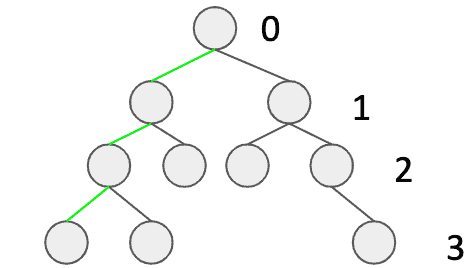
We can find an example of a balanced binary tree below. Three green edges are a simple visualization of how to determine the height, while the numbers indicate the level.

3. Domain Objects

So, let's start with a class for our tree:

public class Tree {
    private int value;
    private Tree left;
    private Tree right;

    public Tree(int value, Tree left, Tree right) {
        this.value = value;
        this.left = left;
        this.right = right;
    }
}

For the sake of simplicity, let's say each node has an integer value. Note, that if left and right trees are null, then it means our node is a leaf.

Before we introduce our primary method let's see what it should return:

private class Result {
    private boolean isBalanced;
    private int height;

    private Result(boolean isBalanced, int height) {
        this.isBalanced = isBalanced;
        this.height = height;
    }
}

Thus for every single call, we'll have information about height and balance.

4. Algorithm

Having a definition of a balanced tree, we can come up with an algorithm. What we need to do is to check the desired property for every node. It can be achieved easily with recursive depth-first search traversal.

Now, our recursive method will be invoked for every node. Additionally, it will keep track of the current depth. Each call will return information about height and balance.

Now, let's take a look at our depth-first method:

private Result isBalancedRecursive(Tree tree, int depth) {
    if (tree == null) {
        return new Result(true, -1);
    }

    Result leftSubtreeResult = isBalancedRecursive(tree.left(), depth + 1);
    Result rightSubtreeResult = isBalancedRecursive(tree.right(), depth + 1);

    boolean isBalanced = Math.abs(leftSubtreeResult.height - rightSubtreeResult.height) <= 1;
    boolean subtreesAreBalanced = leftSubtreeResult.isBalanced && rightSubtreeResult.isBalanced;
    int height = Math.max(leftSubtreeResult.height, rightSubtreeResult.height) + 1;

    return new Result(isBalanced && subtreesAreBalanced, height);
}

First, we need to consider the case if our node is null: we'll return true (which means the tree is balanced) and -1 as a height.

Then, we make two recursive calls for the left and the right subtree, keeping the depth up to date.

At this point, we have calculations performed for children of a current node. Now, we have all the required data to check balance:

• the isBalanced variable checks the height for children, and
• substreesAreBalanced indicates if the subtrees are both balanced as well

Finally, we can return information about balance and height. It might be also a good idea to simplify the first recursive call with a facade method:

public boolean isBalanced(Tree tree) {
    return isBalancedRecursive(tree, -1).isBalanced;
}

5. Summary

In this article, we've discussed how to determine if a binary tree is balanced. We've explained a depth-first search approach.

As usual, the source code with tests is available over on GitHub.

1. Introduction

In this short tutorial, we’ll take a look at different FetchMode values we can use in the @org.hibernate.annotations.Fetch annotation.

2. Setting up the Example

As an example, we'll use the following Customer entity with just two properties – an id and a set of orders:

@Entity
public class Customer {

    @Id
    @GeneratedValue
    private Long id;

    @OneToMany(mappedBy = "customer")
    @Fetch(value = FetchMode.SELECT)
    private Set<Order> orders = new HashSet<>();

    // getters and setters
}

Also, we'll create an Order entity consisting of an id, a name and a reference to the Customer.

@Entity
public class Order {

    @Id
    @GeneratedValue
    private Long id;

    private String name;

    @ManyToOne
    @JoinColumn(name = "customer_id")
    private Customer customer;

    // getters and setters
}

In each of the next sections, we'll fetch the customer from the database and get all of its orders:

Customer customer = customerRepository.findById(id).get();
Set<Order> orders = customer.getOrders();

3. FetchMode.SELECT

On our Customer entity, we've annotated the orders property with a @Fetch annotation:

@OneToMany
@Fetch(FetchMode.SELECT)
private Set<Orders> orders;

We use @Fetch to describe how Hibernate should retrieve the property when we lookup a Customer.

Using SELECT indicates that the property should be loaded lazily.

This means that for the first line:

Customer customer = customerRepository.findById(id).get();

We won't see a join with the orders table:

Hibernate: 
    select ...from customer
    where customer0_.id=?

And that for the next line:

Customer customer = customerRepository.findById(id).get();

We'll see subsequent queries for the related orders:

Hibernate: 
    select ...from order
    where order0_.customer_id=?

The Hibernate FetchMode.SELECT generates a separate query for each Order that needs to be loaded.

In our example, that gives one query to load the Customers and five additional queries to load the orders collection.

This is known as the n + 1 select problem. Executing one query will trigger n additional queries.

3.1. @BatchSize

FetchMode.SELECT has an optional configuration annotation using the @BatchSize annotation:

@OneToMany
@Fetch(FetchMode.SELECT)
@BatchSize(size=10)
private Set<Orders> orders;

Hibernate will try to load the orders collection in batches defined by the size parameter.

In our example, we have just five orders so one query is enough.

We'll still use the same query:

Hibernate:
    select ...from order
    where order0_.customer_id=?

But it will only be run once. Now we have just two queries: One to load the Customer and one to load the orders collection.

4. FetchMode.JOIN

While FetchMode.SELECT loads relations lazily, FetchMode.JOIN loads them eagerly, say via a join:

@OneToMany
@Fetch(FetchMode.JOIN)
private Set<Orders> orders;

This results in just one query for both the Customer and their Orders:

Hibernate: 
    select ...
    from
        customer customer0_ 
    left outer join
        order order1 
            on customer.id=order.customer_id 
    where
        customer.id=?

5. FetchMode.SUBSELECT

Because the orders property is a collection, we could also use FetchMode.SUBSELECT:

@OneToMany
@Fetch(FetchMode.SUBSELECT)
private Set<Orders> orders;

We can only use SUBSELECT with collections.

With this setup, we go back to one query for the Customer:

Hibernate: 
    select ...
    from customer customer0_

And one query for the Orders, using a sub-select this time:

Hibernate: 
    select ...
    from
        order order0_ 
    where
        order0_.customer_id in (
            select
                customer0_.id 
            from
                customer customer0_
        )

6. FetchMode vs. FetchType

In general, FetchMode defines how Hibernate will fetch the data (by select, join or subselect). FetchType, on the other hand, defines whether Hibernate will load data eagerly or lazily.

The exact rules between these two are as follows:

• if the code doesn't set FetchMode, the default one is JOIN and FetchType works as defined
  
• with FetchMode.SELECT or FetchMode.SUBSELECT set, FetchType also works as defined
• with FetchMode.JOIN set, FetchType is ignored and a query is always eager

For further information please refer to Eager/Lazy Loading In Hibernate.

7. Conclusion

In this tutorial, we’ve learned about FetchMode‘s different values and also how they are related to FetchType.

As always all source code is available on GitHub.

1. Overview

In this tutorial, we'll see different algorithms allowing us to find the smallest missing positive integer in an array. First, we'll go through the explanation of the problem. After that, we'll see three different algorithms suiting our needs. Finally, we'll discuss their complexities.

2. Problem Explanation

First, let's explain what the goal of the algorithm is. We want to search for the smallest missing positive integer in an array of positive integers. That is, in an array of x elements, find the smallest element between 0 and x – 1 that is not in the array. If the array contains them all, then the solution is x, the array size.

For example, let's consider the following array: [0, 1, 3, 5, 6]. It has 5 elements. That means we're searching for the smallest integer between 0 and 4 that is not in this array. In this specific case, it's 2.

Now, let's imagine another array: [0, 1, 2, 3]. As it has 4 elements, we're searching for an integer between 0 and 3. None is missing, thus the smallest integer that is not in the array is 4.

3. Sorted Array

Now, let's see how to find the smallest missing number in a sorted array. In a sorted array, the smallest missing integer would be the first index that doesn't hold itself as a value.

Let's consider the following sorted array: [0, 1, 3, 4, 6, 7]. Now, let's see which value matches which index:

Index: 0 1 2 3 4 5
Value: 0 1 3 4 6 7

As we can see, the value index doesn't hold integer 2, therefore 2 is the smallest missing integer in the array.

How about implementing this algorithm in Java? Let's first create a class SmallestMissingPositiveInteger with a method searchInSortedArray():

public class SmallestMissingPositiveInteger {
    public static int searchInSortedArray(int[] input) {
        // ...
    }
}

Now, we can iterate over the array and search for the first index that doesn't contain itself as a value and return it as the result:

for (int i = 0; i < input.length; i++) {
    if (i != input[i]) {
        return i;
    }
}

Finally, if we complete the loop without finding a missing element, we must return the next integer, which is the array length, as we start at index 0:

return input.length;

Let's check that this all works as expected. Imagine an array of integers from 0 to 5, with the number 3 missing:

int[] input = new int[] {0, 1, 2, 4, 5};

Then, if we search for the first missing integer, 3 should be returned:

int result = SmallestMissingPositiveInteger.searchInSortedArray(input);

assertThat(result).isEqualTo(3);

But, if we search for a missing number in an array without any missing integer:

int[] input = new int[] {0, 1, 2, 3, 4, 5};

We'll find that the first missing integer is 6, which is the length of the array:

int result = SmallestMissingPositiveInteger.searchInSortedArray(input);

assertThat(result).isEqualTo(input.length);

Next, we'll see how to handle unsorted arrays.

4. Unsorted Array

So, what about finding the smallest missing integer in an unsorted array? There are multiple solutions. The first one is to simply sort the array first and then reuse our previous algorithm. Another approach would be to use another array to flag the integers that are present and then traverse that array to find the first one missing.

4.1. Sorting the Array First

Let's start with the first solution and create a new searchInUnsortedArraySortingFirst() method.

So, we'll be reusing our algorithm, but first, we need to sort our input array. In order to do that, we'll make use of Arrays.sort():

Arrays.sort(input);

That method sorts its input according to its natural order. For integers, that means from the smallest to the greatest one. There are more details about sorting algorithms in our article on sorting arrays in Java.

After that, we can call our algorithm with the now sorted input:

return searchInSortedArray(input);

That's it, we can now check that everything works as expected. Let's imagine the following array with unsorted integers and missing numbers 1 and 3:

int[] input = new int[] {4, 2, 0, 5};

As 1 is the smallest missing integer, we expect it to be the result of calling our method:

int result = SmallestMissingPositiveInteger.searchInUnsortedArraySortingFirst(input);

assertThat(result).isEqualTo(1);

Now, let's try it on an array with no missing number:

int[] input = new int[] {4, 5, 1, 3, 0, 2};

int result = SmallestMissingPositiveInteger.searchInUnsortedArraySortingFirst(input);

assertThat(result).isEqualTo(input.length);

That's it, the algorithm returns 6, that is the array length.

4.2. Using a Boolean Array

Another possibility is to use another array – having the same length as the input array – that holds boolean values telling if the integer matching an index has been found in the input array or not.

First, let's create a third method, searchInUnsortedArrayBooleanArray().

After that, let's create the boolean array, flags, and for each integer in the input array that matches an index of the boolean array, we set the corresponding value to true:

boolean[] flags = new boolean[input.length];
for (int number : input) {
    if (number < flags.length) {
        flags[number] = true;
    }
}

Now, our flags array holds true for each integer present in the input array, and false otherwise. Then, we can iterate over the flags array and return the first index holding false. If none, we return the array length:

for (int i = 0; i < flags.length; i++) {
    if (!flags[i]) {
        return i;
    }
}

return flags.length;

Again, let's try this algorithm with our examples. We'll first reuse the array missing 1 and 3:

int[] input = new int[] {4, 2, 0, 5};

Then, when searching for the smallest missing integer with our new algorithm, the answer is still 1:

int result = SmallestMissingPositiveInteger.searchInUnsortedArrayBooleanArray(input);

assertThat(result).isEqualTo(1);

And for the complete array, the answer doesn't change either and is still 6:

int[] input = new int[] {4, 5, 1, 3, 0, 2};

int result = SmallestMissingPositiveInteger.searchInUnsortedArrayBooleanArray(input);

assertThat(result).isEqualTo(input.length);

5. Complexities

Now that we've covered the algorithms, let's talk about their complexities, using Big O notation.

5.1. Sorted Array

Let's start with the first algorithm, for which the input is already sorted. In this case, the worst-case scenario is not finding a missing integer and, therefore, traversing the entire array. This means we have linear complexity, which is noted O(n), considering n is the length of our input.

5.2. Unsorted Array with Sorting Algorithm

Now, let's consider our second algorithm. In this case, the input array is not sorted, and we sort it before applying the first algorithm. Here, the complexity will be the greatest between that of the sorting mechanism and that of the algorithm itself.

As of Java 11, the Arrays.sort() method uses a dual-pivot quick-sort algorithm to sort arrays. The complexity of this sorting algorithm is, in general, O(n log(n)), though it could degrade up to O(n²). That means the complexity of our algorithm will be O(n log(n)) in general and can also degrade up to a quadratic complexity of O(n²).

That's for time complexity, but let's not forget about space. Although the search algorithm doesn't take extra space, the sorting algorithm does. Quick-sort algorithm takes up to O(log(n)) space to execute. That's something we may want to consider when choosing an algorithm for large arrays.

5.3. Unsorted Array with Boolean Array

Finally, let's see how our third and last algorithm performs. For this one, we don't sort the input array, which means we don't suffer the complexity of sorting. As a matter of fact, we only traverse two arrays, both of the same size. That means our time complexity should be O(2n), which is simplified to O(n). That's better than the previous algorithm.

But, when it comes to space complexity, we're creating a second array of the same size as the input. That means we have O(n) space complexity, which is worse than the previous algorithm.

Knowing all that, it's up to us to choose an algorithm that best suits our needs, depending on the conditions in which it'll be used.

6. Conclusion

In this article, we've looked at algorithms for finding the smallest missing positive integer in an array. We've seen how to achieve that in a sorted array, as well as in an unsorted array. We also discussed the time and space complexities of the different algorithms, allowing us to choose one wisely according to our needs.

As usual, the complete code examples shown in this article are available over on GitHub.

1. Introduction

By default, the floating-point computations in Java are platform-dependent. And so, the floating-point outcome's precision depends on the hardware in-use.

In this tutorial, we'll learn how to use strictfp in Java to ensure platform-independent floating-point computations.

2. strictfp Usage

We can use the strictfp keyword as a non-access modifier for classes, non-abstract methods or interfaces:

public strictfp class ScientificCalculator {
    ...
    
    public double sum(double value1, double value2) {
        return value1 + value2;
    }

    public double diff(double value1, double value2) { 
        return value1 - value2; 
    }
}

public strictfp void calculateMarksPercentage() {
    ...
}

public strictfp interface Circle {
    double computeArea(double radius);
}

When we declare an interface or a class with strictfp, all of its member methods and other nested types inherit its behavior.

However, please note that we're not allowed to use strictfp keyword on variables, constructors or abstract methods.

Additionally, for cases when we have a superclass marked with it, it won't make our subclass inherit that behavior.

3. When to Use?

Java strictfp keyword comes handy whenever we care a great deal about the deterministic behavior of all floating-point computations:

@Test
public void whenMethodOfstrictfpClassInvoked_thenIdenticalResultOnAllPlatforms() {
    ScientificCalculator calculator = new ScientificCalculator();
    double result = calculator.sum(23e10, 98e17);
    assertThat(result, is(9.800000230000001E18));

    result = calculator.diff(Double.MAX_VALUE, 1.56);
    assertThat(result, is(1.7976931348623157E308));
}

Since the ScientificCalculator class makes use of this keyword, the above test case will pass on all hardware platforms. Please note that if we don't use it, JVM is free to use any extra precision available on the target platform hardware.

A popular real-world use-case for it is a system performing highly-sensitive medicinal calculations.

4. Conclusion

In this quick tutorial, we talked about when and how to use the strictfp keyword in Java.

As usual, all the presented code samples are available over on GitHub.

1. Overview

Encryption is the process of encoding data with the intent of keeping it safe from unauthorized access.

In this quick tutorial, we'll learn how to encrypt and decrypt files in Linux systems using GPG (GNU Privacy Guard), which is popular and free software.

2. Basics of Encryption

Before we start, let's try to understand some basic concepts.

Basically, all types of encryption (and decryption) primarily involve either a passphrase or a key, which are simply data strings.

2.1. Types of Encryption

Depending on the number of data strings involved in the encryption and decryption process, we have two kinds of encryption.

When only one data string – a passphrase – is used for both encryption and decryption, it's called symmetric encryption. We generally use symmetric encryption when we don't need to share the encrypted files with anyone else. If we do share, then we'd need to share the passphrase as well, which can be a potential risk factor.

On the other hand, when two data strings are involved, one for encryption and another for decryption, it's called asymmetric encryption. Accordingly, the pair of data strings are called key pairs.

Asymmetric encryption is more suitable for the sharing of encrypted files, as it requires sharing only one of the two data strings. We'll discuss this later in the tutorial.

2.2. Types of Keys

In asymmetric encryption, a key pair consists of two keys — a public key and a private key.

The public key is not confidential. Therefore, we can share the public key with stakeholders without any risk.

On the contrary, we should always keep the private key a secret and never share it with anyone.

Public keys are always used for encryption and private keys for decryption when it comes to data encryption/decryption.

It might be worthwhile to know that public/private keys can also be used in the field of digital signatures. In such cases, we use the private key to create the signature and its corresponding public key to verify its authenticity.

3. GPG Installation

Let's open a terminal window and check if GPG is installed:

> gpg --version
gpg (GnuPG) 2.2.4

If it's not installed, let's go ahead and install it using the package manager of our Linux distribution.

For apt based distributions:

> sudo apt install gnupg

Or, for yum based distributions:

> sudo yum install gnupg

The GPG tool comes with both GUI and CLI, but we'll be using the command line for our examples.

Additionally, we'll be using the appropriate options to run the commands in unattended mode.

4. Symmetric Encryption

4.1. Encrypting Files

Let's now try encrypting a file by first creating a sample file:

> echo "Hello, Baeldung!" > greetings.txt

Next, let's run the gpg command to encrypt the file using a passphrase:

> gpg --batch --output greetings.txt.gpg --passphrase mypassword --symmetric greetings.txt

Subsequently, this will create the encrypted file greetings.txt.gpg in the same location using the default AES256 algorithm. To use a different algorithm, we can use the option —cipher-algo.

4.2. Decrypting Files

Let's now try to decrypt the encrypted file from the previous example:

> gpg --batch --output greetings1.txt --passphrase mypassword --decrypt greetings.txt.gpg
gpg: AES256 encrypted data
gpg: encrypted with 1 passphrase

This will create the decrypted file greetings1.txt in the same location.

Note that if we omit the –batch option, the system prompts us to enter the passphrase and then stores it in the session.

Therefore, to clear the password stored in the session, we can run:

echo RELOADAGENT | gpg-connect-agent

Let's now get back to our decrypted file and verify that the decryption was successful:

> diff -s greetings.txt greetings1.txt
Files greetings.txt and greetings1.txt are identical

5. Asymmetric Encryption

In this type of encryption, there are two roles involved — a sender and a receiver.

The receiver decrypts the received file. Thus, the receiver is responsible for generating the key pair. Above all, the receiver would safely keep the private key secret and share only the public key with the sender.

The sender encrypts the file to be sent using the public key shared by the receiver.

Let's see how this works using an example where Ryan is the receiver, and Sam is the sender.

To simplify things, let's create two work folders for each of them, which, in the real-world, would represent two different systems:

> mkdir ryan
> mkdir sam

5.1. Generating a Public/Private Key Pair

The first step is for Ryan, as the receiver, to generate a key pair in his folder:

> cd ryan
> gpg --batch --generate-key <<EOF
    Key-Type: RSA
    Key-Length: 3072
    Subkey-Type: RSA
    Subkey-Length: 3072
    Name-Real: Ryan
    Name-Email: ryan@somewhere.com
    Passphrase: ryanpassword
    Expire-Date: 30
    %pubring ryanpubring.kbx
    %commit
EOF

This will generate the key pair and store it in the ryanpubring.kbx keyring file in the same location.

Let's view the public key entry made to the keyring file:

> gpg --keyring ./ryanpubring.kbx --no-default-keyring --list-keys

./ryanpubring.kbx
-----------------
pub   rsa3072 2019-10-27 [SCEA] [expires: 2019-11-26]
      120C528F1D136BCF7AAACEE6D6BA055613B064D7
uid           [ unknown] Ryan <ryan@somewhere.com>
sub   rsa3072 2019-10-27 [SEA] [expires: 2019-11-26]

The pub indicator is for the public key.

Similarly, we can view the private key entry:

> gpg --keyring ./ryanpubring.kbx --no-default-keyring --list-secret-keys

./ryanpubring.kbx
-----------------
sec   rsa3072 2019-10-27 [SCEA] [expires: 2019-11-26]
      120C528F1D136BCF7AAACEE6D6BA055613B064D7
uid           [ultimate] Ryan <ryan@somewhere.com>
ssb   rsa3072 2019-10-27 [SEA] [expires: 2019-11-26]

Here, sec indicates that this is a secret or private key.

5.2. Sharing Public Key

After a successful key generation, Ryan can export the public key from his keyring into a file:

> gpg --keyring ./ryanpubring.kbx --no-default-keyring --armor --output ryanpubkey.gpg --export ryan@somewhere.com

This will generate a new file ryanpubkey.gpg containing the public key. Let's take a peek at the file content:

> cat ryanpubkey.gpg
-----BEGIN PGP PUBLIC KEY BLOCK-----
mQGNBF21KQoBDACs7bgjl22TPyQDKjLTMlZrBgQrXZOIkNcH3z1f87XQYoLjVPU3
ymg1hweHm1RsIxO+GdD42pkU/ob5YdWgvVBRdIZPeTXciTa8TtxZKNNtr+IL0pwY
...
-----END PGP PUBLIC KEY BLOCK-----

Ryan can now share this file with Sam via secured or unsecured channels.

In our example, let's do a simple file copy for sharing the public key:

> cp ryanpubkey.gpg ../sam

5.3. Importing Public Key

Let's now see what Sam has to do after receiving the public key from Ryan.

First, let's switch to Sam's folder:

> cd ../sam

Then, let's import Ryan's public key into Sam's keyring file:

> gpg --keyring ./sampubring.kbx --no-default-keyring --import ryanpubkey.gpg
gpg: keybox './sampubring.kbx' created
gpg: key D6BA055613B064D7: public key "Ryan <ryan@somewhere.com>" imported
gpg: Total number processed: 1
gpg:               imported: 1
gpg: public key of ultimately trusted key 01220F5773165740 not found
gpg: marginals needed: 3  completes needed: 1  trust model: pgp
gpg: depth: 0  valid:   2  signed:   0  trust: 0-, 0q, 0n, 0m, 0f, 2u
gpg: next trustdb check due at 2019-11-26

This will create a new keyring file sampubring.kbx and add the public key to it.

We can now view the imported key:

> gpg --keyring ./sampubring.kbx --no-default-keyring --list-keys
...
uid           [ unknown] Ryan <ryan@somewhere.com>

The [ unknown] indicates that information regarding the key's trustworthiness is not available. To avoid warnings in the future, let's change this to trusted:

> gpg --keyring ./sampubring.kbx --no-default-keyring --edit-key "ryan@somewhere.com" trust

In the trust level question that is asked, let's specify our choice as 5 = I trust ultimately and confirm as yes. After that, let's type quit to exit from the shell.

5.4. Encrypting Files

Sam is now all set to encrypt a file that only Ryan can read. Let's create a sample file:

> echo "Hello, Baeldung!" > greetings.txt

Afterward, let's specify Ryan as the recipient in the encrypt command:

> gpg --keyring ./sampubring.kbx --no-default-keyring --encrypt --recipient "ryan@somewhere.com" greetings.txt

This creates the file greetings.txt.gpg in the same location and encrypted using Ryan's public key. Sam can now share this file with Ryan via secured or unsecured channels.

As before, let's do a simple file copy for sharing the encrypted file:

> cp greetings.txt.gpg  ../ryan

5.5. Decrypting Files

Let's now return to Ryan's folder to read the encrypted file he received from Sam:

> cd ../ryan

We can use the decrypt command:

> gpg --keyring ./ryanpubring.kbx --no-default-keyring --pinentry-mode=loopback --passphrase "ryanpassword" --output greetings.txt --decrypt greetings.txt.gpg
gpg: encrypted with 3072-bit RSA key, ID 8273FAC75696D83E, created 2019-10-27
      "Ryan <ryan@somewhere.com>"

This will create a new file greetings.txt decrypted using Ryan's private key.

We can quickly check if decryption was successful:

> diff -s greetings.txt ../sam/greetings.txt
Files greetings.txt and ../sam/greetings.txt are identical

5.6. Two-Way Communications

In the previous example, the communication is unidirectional, as the sender and receiver roles are static.

What this means is that for enabling bidirectional communication, all we need to do is reverse the roles by generating a second key pair. We can follow the same steps listed in the previous section.

6. Conclusion

In this article, we learned how to encrypt files using two different approaches so that, depending on the requirement, we can decide upon the most suitable one for the task.

We also learned about public/private keys and how to use them practically for file encryption/decryption.

1. Spring and Java

>> Static Data with Spring Boot [reflectoring.io]

A good tutorial on externalizing application configuration with @ConfigurationProperties.

>> The best way to fix the Hibernate MultipleBagFetchException [vladmihalcea.com]

A quick look at the right way to solve this problem, while exposing inefficiencies of an often-recommended approach.

>> Easier attribute management in Java EE [blog.frankel.ch]

And a trip down memory lane shows how request/session attribute management has changed since J2EE.

Also worth reading:

• >> Spring Cloud Gateway with OpenID Connect and Token Relay [blog.jdriven.com]

• >> Microservices with Spring Boot, Spring Cloud Gateway and Consul Cluster [piotrminkowski.wordpress.com]

• >> Tutorial: Reactive Spring Boot Part 3 – A JavaFX Spring Boot Application [blog.jetbrains.com]

• >> Hibernate Tip: How to integrate an external query builder [thoughts-on-java.org]

• >> Improving CompletableFuture#allOf/anyOf API Java Methods [4comprehension.com]

• >> Configuring A Quarkus Application With Profiles [antoniogoncalves.org]

Webinars and presentations:

• >> A Bootiful Podcast: Michael Simons on Spring Boot, reactive Spring Data Neo4j, and more [spring.io]

• >> Java on Azure: Building Spring Boot microservices [myignite.techcommunity.microsoft.com]

• >> Clean Code: The Next Chapter by Victor Rentea [youtube.com]

• >> Why We Hate Java Serialization And What We're Doing About It by Brian Goetz & Stuart Marks [youtube.com]

• >> Qualities of a Highly Effective Architect Keynote by Venkat Subramaniam [youtube.com]

• >> Java 12 & 13 What's new and noteworthy? By Piotr Przybyl [youtube.com]

• >> Java 9 and Beyond by Venkat Subramaniam [youtube.com]

• >> Reactive Revolution by Josh Long [youtube.com]

Time to upgrade:

• >> Spring Boot 2.2.1 available now [spring.io] and >> Spring Boot 2.1.10 available now [spring.io]

• >> Spring Boot for Apache Geode & Pivotal GemFire 1.1.3.RELEASE & 1.2.1.RELEASE Available [spring.io]

• >> Spring Vault 2.2 goes GA  [spring.io]

• >> Spring Integration Extensions Releases [spring.io]

• >> Gradle 6.0 Release Notes [docs.gradle.org]

2. Technical and Musings

>> AWS CDK Part 3: How to create an RDS instance [blog.codecentric.de] and >> AWS CDK Part 4: How to create Lambdas [blog.codecentric.de]

A couple of tutorials show how to a set up an AWS relational database service and interact with it from Lambdas.

>> Stackbit: build JAMStack sites in a few clicks [vojtechruzicka.com]

And a new tool for building static sites integrates seamlessly with site generators and CMS.

Also worth reading:

• >> Seamless S3 encryption does not imply better security [advancedweb.hu]

• >> Open Source, SaaS and Monetization [lucumr.pocoo.org]

3. Comics

And my favorite Dilberts of the week:

>> Multiple Choice [dilbert.com]

>> Wally Compared to a Placebo [dilbert.com]

>> Workflow Training [dilbert.com]

4. Pick of the Week

>> Google Interview Problems: Ratio Finder [medium.com]

1. Overview

Our builds often run a lot of automated test cases for our project. These include unit and integration tests. If the execution of the test suite takes a long time, we may wish to optimize our test code or track down tests that are taking too long.

In this tutorial, we'll learn a few ways to determine the execution time of our test cases and test suites.

2. JUnit Examples

To demonstrate reporting execution times, let's use some example test cases from different layers of the test pyramid. We'll simulate the test case duration with Thread.sleep().

We'll implement our examples in JUnit 5. However, the equivalent tools and techniques also apply to test cases written with JUnit 4.

First, here's a trivial unit test:

@Test
void someUnitTest() {

    assertTrue(doSomething());
}

Second, let's have an integration test that takes more time to execute:

@Test
void someIntegrationTest() throws Exception {

    Thread.sleep(5000);
    assertTrue(doSomething());
}

Finally, we can simulate a slow end-to-end user scenario:

@Test
void someEndToEndTest() throws Exception {

    Thread.sleep(10000);
    assertTrue(doSomething());
}

In the rest of the article, we'll execute these test cases and determine their execution times.

3. IDE JUnit Runner

The quickest way to find the execution time of a JUnit test is to use our IDE. Since most IDEs come with embedded JUnit runner, they execute and report the test results.

The two most popular IDEs, IntelliJ and Eclipse, have embedded JUnit runners.

2.1. IntelliJ JUnit Runner

IntelliJ allows us to execute JUnit test cases with the help of run/debug configurations. Once we execute the tests, the runner shows the test status along with the execution time:

Since we executed all three of our example test cases, we can see the total execution time as well as the time taken by each test case.

We may also need to save such reports for future reference. IntelliJ allows us to export this report in either HTML or XML format. The export report function is highlighted on the toolbar in the screenshot above.

2.2. Eclipse JUnit Runner

Eclipse also provides an embedded JUnit runner. We can execute and find out the execution time of a single test case or an entire test suite in the test results window:

But, in contrast to the IntelliJ test runner, we cannot export a report from Eclipse.

3. Maven Surefire Plugin

The Maven Surefire plugin is used to execute unit tests during the test phase of the build lifecycle. The surefire plugin is part of the default Maven configuration. However, if a specific version or additional configuration is required, we can declare it in the pom.xml:

<plugin>
    <groupId>org.apache.maven.plugins</groupId>
    <artifactId>maven-surefire-plugin</artifactId>
    <version>3.0.0-M3</version>
    <configuration>
        <excludes>
            <exclude>**/*IntegrationTest.java</exclude>
        </excludes>
    </configuration>
    <dependencies>
        <dependency>
            <groupId>org.junit.platform</groupId>
            <artifactId>junit-platform-surefire-provider</artifactId>
            <version>1.3.2</version>
        </dependency>
    </dependencies>
</plugin>

There are three ways to find the execution time of JUnit tests when testing with Maven. We'll examine each one in the next subsections.

3.1. Maven Build Logs

Surefire displays the execution status and time of every test case in the build logs:

[INFO] Running com.baeldung.execution.time.SampleExecutionTimeUnitTest
[INFO] Tests run: 3, Failures: 0, Errors: 0, Skipped: 0, Time elapsed: 15.003 s 
- in com.baeldung.execution.time.SampleExecutionTimeUnitTest

Here, it shows the combined execution time of all three test cases in the test class.

3.2. Surefire Test Reports

The surefire plugin also generates a test execution summary in .txt and .xml formats. These are generally stored in the target directory of the project. Surefire follows a standard format for both text reports:

----------------------------------------------
Test set: com.baeldung.execution.time.SampleExecutionTimeUnitTest
----------------------------------------------
Tests run: 3, Failures: 0, Errors: 0, Skipped: 0, Time elapsed: 15.003 s 
- in com.baeldung.execution.time.SampleExecutionTimeUnitTest

and XML reports:

<?xml version="1.0" encoding="UTF-8"?>
<testsuite
	xmlns:xsi="http://www.w3.org/2001/XMLSchema-instance"
	xsi:noNamespaceSchemaLocation="https://maven.apache.org/surefire/maven-surefire-plugin/xsd/surefire-test-report.xsd"
	name="com.baeldung.execution.time.SampleExecutionTimeUnitTest"
	time="15.003" tests="3" errors="0" skipped="0" failures="0">
	<testcase name="someEndToEndTest"
		classname="com.baeldung.execution.time.SampleExecutionTimeUnitTest"
		time="9.996" />
	<testcase name="someIntegrationTest"
		classname="com.baeldung.execution.time.SampleExecutionTimeUnitTest"
		time="5.003" />
	<testcase name="someUnitTest"
		classname="com.baeldung.execution.time.SampleExecutionTimeUnitTest"
		time="0.002" />
</testsuite>

Although the text format is more suited for readability, the XML format is machine-readable and can be imported for visualization in HTML and other tools.

3.3. Surefire HTML Reports

We can view our test report in HTML in our browser by using the maven-surefire-report-plugin:

<reporting>
    <plugins>
        <plugin>
            <groupId>org.apache.maven.plugins</groupId>
            <artifactId>maven-surefire-report-plugin</artifactId>
            <version>3.0.0-M3</version>
        </plugin>
    </plugins>
</reporting>

We can now execute mvn commands to generate the report:

1. mvn surefire-report:report – executes the tests and generates an HTML report
2. mvn site – adds CSS styling to the HTML generated in the last step

This report shows the execution time of all the test cases in a class or a package along with the time taken by each test case.

4. Jenkins Test Results

If we are running CI in Jenkins, we can import the XML files written by surefire. This allows Jenkins to mark a build as failed if the tests fail, and to show us test trends and results.

When we review the test results in Jenkins, we also see the execution times.

For our example, after installing Jenkins, we'll configure a job using Maven and the surefire XML report files to publish the test results:

We added a post-build action in our job to publish the test results. Jenkins will now import the XML files from the given path and add this report to the build execution summary:

This can also be achieved using Jenkins pipeline builds.

5. Conclusion

In this article, we discussed various ways of determining the execution time of JUnit tests. The most immediate method is to use our IDE's JUnit runner.

We then used the maven-surefire-plugin to archive the test reports in text, XML, and HTML formats.

Finally, we provided our test report output to our CI server, which can help us analyze how different builds performed.

As always, the example code from this article is available over on GitHub.

1. Overview

In this short tutorial, we'll investigate the definition of “Plain Old Java Object” or POJO for short.

We'll look at how a POJO compares to a JavaBean, and how turning our POJOs into JavaBeans can be helpful.

2. Plain Old Java Objects

2.1. What is a POJO

When we talk about a POJO, what we're describing is a straightforward type with no references to any particular frameworks. A POJO has no naming convention for our properties and methods.

Let's create a basic employee POJO. It'll have three properties; first name, last name, and start date:

public class EmployeePojo {

    public String firstName;
    public String lastName;
    private LocalDate startDate;

    public EmployeePojo(String firstName, String lastName, LocalDate startDate) {
        this.firstName = firstName;
        this.lastName = lastName;
        this.startDate = startDate;
    }

    public String name() {
        return this.firstName + " " + this.lastName;
    }

    public LocalDate getStart() {
        return this.startDate;
    }
}

This class can be used by any Java program as it's not tied to any framework.

But, we aren't following any real convention for constructing, accessing, or modifying the class's state.

This lack of convention causes two problems:

First, it increases the learning curve for coders trying to understand how to use it.

Second, it may limit a framework's ability to favor convention over configuration, understand how to use the class, and augment its functionality.

To explore this second point, let's work with EmployeePojo using reflection. Thus, we'll start to find some of its limitations.

2.2. Reflection with a POJO

Let's add the commons-beanutils dependency to our project:

<dependency>
    <groupId>commons-beanutils</groupId>
    <artifactId>commons-beanutils</artifactId>
    <version>1.9.4</version>
</dependency>

And now, let's inspect the properties of our POJO:

List<String> propertyNames =
  PropertyUtils.getPropertyDescriptors(EmployeePojo.class).stream()
    .map(PropertyDescriptor::getDisplayName)
    .collect(Collectors.toList());

If we were to print out propertyNames to the console, we'd only see:

[start]

Here, we see that we only get start as a property of the class. PropertyUtils failed to find the other two.

We'd see the same kind of outcome were we to use other libraries like Jackson to process EmployeePojo.

Ideally, we'd see all our properties: firstName, lastName, and startDate. And the good news is that many Java libraries support by default something called the JavaBean naming convention.

3. JavaBeans

3.1. What is a JavaBean?

A JavaBean is still a POJO but introduces a strict set of rules around how we implement it:

• Access levels – our properties are private and we expose getters and setters
• Method names – our getters and setters follow the getX and setX convention (in the case of a boolean, isX can be used for a getter)
• Default Constructor – a no-argument constructor must be present so an instance can be created without providing arguments, for example during deserialization
• Serializable – implementing the Serializable interface allows us to store the state

3.2. EmployeePojo as a JavaBean

So, let's try converting EmployeePojo into a JavaBean:

public class EmployeeBean implements Serializable {

    private static final long serialVersionUID = -3760445487636086034L;
    private String firstName;
    private String lastName;
    private LocalDate startDate;

    public EmployeeBean() {
    }

    public EmployeeBean(String firstName, String lastName, LocalDate startDate) {
        this.firstName = firstName;
        this.lastName = lastName;
        this.startDate = startDate;
    }

    public String getFirstName() {
        return firstName;
    }

    public void setFirstName(String firstName) {
        this.firstName = firstName;
    }

    //  additional getters/setters

}

3.3. Reflection with a JavaBean

When we inspect our bean with reflection, now we get the full list of the properties:

[firstName, lastName, startDate]

4. Tradeoffs When Using JavaBeans

So, we've shown a way in which JavaBeans are helpful. Keep in mind that every design choice comes with tradeoffs.

When we use JavaBeans we should also be mindful of some potential disadvantages:

• Mutability – our JavaBeans are mutable due to their setter methods – this could lead to concurrency or consistency issues
• Boilerplate – we must introduce getters for all properties and setters for most, much of this might be unnecessary
• Zero-argument Constructor – we often need arguments in our constructors to ensure the object gets instantiated in a valid state, but the JavaBean standard requires us to provide a zero-argument constructor

Given these tradeoffs, frameworks have also adapted to other bean conventions over the years.

5. Conclusion

In this tutorial, we compared POJOs with JavaBeans.

First, we learned a POJO is a Java object that is bound to no specific framework, and that a JavaBean is a special type of POJO with a strict set of conventions.

Then, we saw how some frameworks and libraries harness the JavaBean naming convention to discover a class's properties.

As usual, the examples are available over on GitHub.

1. Overview

In this tutorial, we'll look at the implications of catching Throwable.

2. The Throwable Class

In the Java documentation, the Throwable class is defined as “the super-class of all errors and exceptions in the Java language“.

Let's look at the hierarchy of the Throwable class:

The Throwable class has two direct sub-classes – namely, the Error and Exception classes.

Error and its sub-classes are unchecked exceptions, while the sub-classes of Exception can be either checked or unchecked exceptions.

Let's look at the types of situations a program can experience when it fails.

3. Recoverable Situations

There are situations where recovery is generally possible and can be handled with either checked or unchecked sub-classes of the Exception class.

For example, a program might want to use a file that happens to not exist at the specified location, resulting in a checked FileNotFoundException being thrown.

Another example is the program attempting to access a system resource without having permission to do that, resulting in an unchecked AccessControlException being thrown.

As per the Java documentation, the Exception class “indicates conditions that a reasonable application might want to catch“.

4. Irrecoverable Situations

There are cases where a program can get in a state where recovery is impossible in an event of a failure. Common examples of this are when a stack overflow occurs or the JVM runs out of memory.

In these situations, the JVM throws StackOverflowError and OutOfMemoryError, respectively. As suggested by their names, these are sub-classes of the Error class.

According to the Java documentation, the Error class “indicates serious problems that a reasonable application should not try to catch“.

5. Example of Recoverable and Irrecoverable Situations

Let's assume that we have an API that allows callers to add unique IDs to some storage facility using the addIDsToStorage method:

class StorageAPI {

    public void addIDsToStorage(int capacity, Set<String> storage) throws CapacityException {
        if (capacity < 1) {
            throw new CapacityException("Capacity of less than 1 is not allowed");
        }
        int count = 0;
        while (count < capacity) {
            storage.add(UUID.randomUUID().toString());
            count++;
        }
    }

    // other methods go here ...
}

Several potential failure points can occur when invoking addIDsToStorage:

• CapacityException – A checked sub-class of Exception when passing a capacity value of less than 1
• NullPointerException – An unchecked sub-class of Exception if a null storage value is provided instead of an instance of Set<String>
• OutOfMemoryError – An unchecked sub-class of Error if the JVM runs out of memory before exiting the while loop

The CapacityException and NullPointerException situations are failures the program can recover from, but the OutOfMemoryError is an irrecoverable one.

6. Catching Throwable

Let's assume the user of the API only catches Throwable in the try-catch when calling addIDsToStorage:

public void add(StorageAPI api, int capacity, Set<String> storage) {
    try {
        api.addIDsToStorage(capacity, storage);
    } catch (Throwable throwable) {
        // do something here
    }
}

This means that the calling code is reacting to recoverable and irrecoverable situations in the same way.

The general rule in handling exceptions is that the try-catch block must be as specific as possible in catching exceptions. That is, a catch-all scenario must be avoided.

Catching Throwable in our case violates this general rule. To react to recoverable and irrecoverable situations separately, the calling code would have to inspect the instance of the Throwable object inside the catch block.

The better way would be to use a specific approach in handling exceptions and to avoid trying to deal with irrecoverable situations.

7. Conclusion

In this article, we looked at the implications of catching Throwable in a try-catch block.

As always, the full source code of the example is available over on Github.

1. Overview

Machine learning consists of applying mathematical and statistical approaches to get machines to learn from data. It consists of four big families of techniques:

• Supervised learning
• Semi-supervised learning
• Unsupervised learning
• Reinforcement learning

In this article, we'll explore the purpose of machine learning and when we should use specific techniques. Consequently, we'll find out how they work based on simple examples.

2. Supervised Learning

Supervised learning is a technique consisting of providing labeled data to a machine learning model. The labeled dataset is usually data gathered from experience, also called empirical data. In addition, the data often requires preparation to increase its quality, fill its gaps or simply optimize it for training.

Let's take the following dataset of types of wines as an example:

Now let's see what it looks like after preparation:

We've corrected problems related to the quality of the dataset (missing cells) and optimized it to ease the learning process. For example, we can see that the values red and white have been replaced by digital values.

Depending on the use case, we'll use either classification or regression models.

Let's discover what those terms mean and how to choose which fits best.

2.1. Classification

Firstly, let's assume that we have a dataset of car images. We want to classify those images by type: sedan, truck, van, etc. As a result, for this kind of use case, we want to use a classification model.

This type of model will classify our inputs in one of the predefined and exhaustive classes, in this example by type of car.

But before doing that, we'll feed it a large set of images of cars labeled with the correct output class. This is what we call the training step.

After that, the model will be tested on another set of labeled images that it has never processed before. This step is crucial to know how the model behaves given new data to work with.

Finally, we can consider the model mature if the results are reaching a certain level of correct prediction. The level usually depends on the cruciality of the use case. For example, a model filtering out spam is less crucial than a model operating an automated vehicle. We calculate the accuracy of a model using a loss function.

As an illustration, the image hereunder is an example of a classification model consisting of two classes: cat and not a cat:

Let's list some of the algorithms used for classification:

• Logistic regression
• Random forest
• Decision tree
• Support vector regressor
• k-nearest neighbors

2.2. Regression

On the other hand, regression will not give a class as output but a specific value also called a forecast or prediction.

We use regression models to predict those values based on historical data. In that way, it's not much different than the classification model. It also requires a training step and a test step.

For instance, let's say we have the ages of people and their respective height. Using this data, we'll be able to build a model predicting what someone's height is most likely to be, based on their age:

Let's see what algorithms can be used for regression:

• Linear regression
• Random forest
• Decision tree
• Support vector regressor
• k-nearest neighbors

We notice that most of them were also listed in the classification subsection.

3. Unsupervised Learning

In contrast with supervised learning, unsupervised learning consists of working with unlabeled data. In fact, the labels in these use cases are often difficult to obtain. For instance, there is not enough knowledge of the data or the labeling is too expensive.

Moreover, the lack of labels makes it difficult to set goals for the trained model. It's therefore complicated to measure whether results are accurate. Even though that is the case, multiple techniques allow obtaining results that lead to obtaining a better grip on the data.

3.1. Clustering

Clustering consists of discovering clusters of similar items based on some of their features. In other words, this technique helps in revealing patterns in data.

For example, we'll say we have inputs consisting of cars. Besides, the dataset is not labeled, we have no idea what their similar features or set of features could lead to as clusters. The clustering model will find patterns. As an illustration, in the case presented below, it finds a way of grouping cars using their respective colors:

Let's discover some clustering algorithms:

• k-means clustering
• Hierarchical clustering

3.2. Dimensionality Reduction

Dimensionality refers to the number of dimensions in a dataset. For example, dimensions can represent features or variables. They describe entities in the dataset.

The goal of this technique is to detect correlations between different dimensions. In other words, it will help us find redundancy in the dataset features and reduce it. As an example, we can think of two features giving the same information in different forms. As a consequence, the algorithm will only keep one of these columns in the compressed subset.

After that, we'll keep only the minimal necessary dimensions needed without losing any crucial information. In the end, this technique helps to get a better dataset, optimizing the further training step:

We can note a non-exhaustive list of dimensionality reduction algorithms:

• Principal component analysis
• Linear discriminant analysis
• Generalized discriminant analysis
• Kernel principal component analysis

4. Semi-supervised Learning

Similarly to supervised and unsupervised learning, semi-supervised learning consists of working with a dataset.

However, datasets in semi-supervised learning are split into two parts: a labeled part and an unlabeled one. This technique is often used when labeling the data or gathering labeled data is too difficult or too expensive. The part of the data labeled can also be of bad quality.

For example, if we take medical imaging to detect cancer, having doctors labeling the dataset is a very expensive task. Moreover, those doctors have other more urgent work to do. For instance, hereunder, we can see that the doctor has labeled part of the dataset and left the other one unlabeled.

Finally, this technique of machine learning has proven to perform good accuracy even if the dataset is partially labeled.

5. Reinforcement Learning

In reinforcement learning, the system learns exclusively from a series of reinforcements. Those can be positive or negative in relation to a system goal. Positive ones are known as “rewards” while on the other hand, we'll call the negative ones “punishments”.

For instance, let's take a model playing a video game. The system gets a reward when it wins more points. But then, if it loses, the model will receive a punishment. As a result, the model can then identify what moves were good in terms of strategy.

The moves' values will then be added to each other to build a short-term strategy as well as a long-term one. As a consequence, the model will learn how to play the game and accumulate the most awards possible.

Finally, the model evolves with each action and reward or per batch of actions and rewards.

Some algorithms for reinforcement learning are:

• SARSA as in State-action-reward-state-action
• Q-learning
• Thompson sampling
• Upper Confidence Bound
• Monte Carlo tree search

6. How to Choose an Appropriate Approach?

The ideal generic algorithm does not exist. Each algorithm has its strengths and weaknesses. Depending on the use case and different factors, we'll choose one or the other algorithm.

Let's take a look at some non-exhaustive points to consider when choosing an algorithm:

• The type of problem – With the problem to solve in mind, we're going to choose an algorithm that has proven to provide good results for similar problems
• The number of samples available – In general, the larger the dataset the better but some algorithms perform well on little dataset too (e.g Naive Bayes, KNeighbors Classifier, Linear SVC, SVR)
• The complexity of the model's algorithm compared to the amount of data used to train it – More precisely, if the algorithm is too complex but has been trained on very few data, it will be too flexible and may end up overfitting
• The expected accuracy – A machine learning model with low accuracy can get trained way faster than another one aiming for minimal loss

7. Conclusion

In conclusion, we've discovered multiple techniques to apply machine learning. We now know these techniques come in different flavors but all have a point in common: they always consist of maths and stats techniques.

1. Overview

In Linux, everything is a file. So, file manipulations – creating a file, removing a directory, etc. – are very common operations in Linux.

In this tutorial, let's see some useful file manipulation commands and learn how to use them.

Note that we'll only focus on the manipulation of files themselves, not their content.

2. The touch Command

The touch command can be used to create files without any content.

To create empty files, we just touch filenames:

$  ls -l
total 0

$  touch file1.txt file2.txt file3.txt
$  ls -l
total 0
-rw-r--r-- 1 kent kent 0 Oct 27 10:50 file1.txt
-rw-r--r-- 1 kent kent 0 Oct 27 10:50 file2.txt
-rw-r--r-- 1 kent kent 0 Oct 27 10:50 file3.txt

Except for creating empty files, the touch command can help us to update the access time and the modification time of a file.

We can use the -a option to update the access time for file.txt:

$  touch -a --date='1992-08-08 17:17:59' file1.txt
$  ls -u --full-time 
total 0
-rw-r--r-- 1 kent kent 0 1992-08-08 17:17:59.000000000 +0200 file1.txt
-rw-r--r-- 1 kent kent 0 2019-10-27 10:50:53.007703818 +0100 file2.txt
-rw-r--r-- 1 kent kent 0 2019-10-27 10:50:53.007703818 +0100 file3.txt

In the above example, we gave the -u option to the ls command in order to show the access time in the file list.

The -m option is for changing the modification time of a file.

For example, let's change the modification time of the file3.txt to some time in the '70s:

$  touch -m --date='1976-11-18 18:19:59' file3.txt
$  ls --full-time
total 0
-rw-r--r-- 1 kent kent 0 2019-10-27 10:50:53.007703818 +0100 file1.txt
-rw-r--r-- 1 kent kent 0 2019-10-27 10:50:53.007703818 +0100 file2.txt
-rw-r--r-- 1 kent kent 0 1976-11-18 18:19:59.000000000 +0100 file3.txt

3. The mkdir Command

touch is handy for creating empty files. To do the same for directories, we use mkdir.

The syntax of the mkdir command is quite similar to the above touch command.

Let's see an example of how to create three directories in one shot:

$  mkdir one two three
$  ls -l
total 0
drwxr-xr-x 2 kent kent 40 Oct 27 11:22 one/
drwxr-xr-x 2 kent kent 40 Oct 27 11:22 three/
drwxr-xr-x 2 kent kent 40 Oct 27 11:22 two/

The mkdir command will complain if the directory we're about to create exists already.

For instance, we'll get an error if we attempt to create another directory called “one”:

$  mkdir one
mkdir: cannot create directory ‘one’: File exists

A very convenient option on the mkdir command is -p. The -p option allows us to create parent directories as necessary and not complain if the directories exist.

Let's create some sub-directories under the existing one directory – we'll list our result with tree:

$  mkdir -p one/one.1/one.1.1  one/one.2/one.2.1
$  tree -d
.
├── one
│   ├── one.1
│   │   └── one.1.1
│   └── one.2
│       └── one.2.1
├── three
└── two

4. The rm Command

The rm command does the opposite of creating files and directories:  It removes them.

To remove files with rm is easy, we just add the filenames we want to remove after the rm command.

For example, let's say want to remove the three .txt files we created earlier with touch:

$  ls
file1.txt  file2.txt  file3.txt
$  rm file1.txt file2.txt file3.txt
$  ls
total 0

By default, rm does not remove directories. We can make use of the -d option to remove empty directories.

In the next example, let's try to remove a directory we just created: two:

$  rm -d two
$  tree -d
.
├── one
│   ├── one.1
│   │   └── one.1.1
│   └── one.2
│       └── one.2.1
└── three

If we apply the same command on the directory one, we'll get an error since the directory one is not empty, it has sub-directories:

$  rm -d one
rm: cannot remove 'one': Directory not empty

If we want to remove directories and their contents recursively, we should use the rm‘s -r option:

$  rm -r one
$  tree -d
.
└── three

The rm command will prompt for confirmation removal if a file is write-protected:

$  ls -l
total 0
drwxr-xr-x 2 kent kent  80 Oct 27 16:55 ./
drwxr-xr-x 5 kent kent 100 Oct 27 11:56 ../
-r--r--r-- 1 kent kent   0 Oct 27 16:55 readOnly1
-r--r--r-- 1 kent kent   0 Oct 27 16:54 readOnly2

$  rm readOnly1
rm: remove write-protected regular empty file 'readOnly1'? y

$  ls -l
total 0
-r--r--r-- 1 kent kent 0 Oct 27 16:54 readOnly2

However the -f option overrides this minor protection and removes the file forcefully.

Let's remove the other write-protected file with the -f option:

$  rm -f readOnly2 
$  ls -l
total 0

The rm command works normally silently. So, we should be very careful while executing the rm command, particularly with the -r and the -f options. Once the files or directories get deleted, it's really hard to recover them again.

5. The cp Command

The cp command is used to copy files or directories.

Let's take a look at how to make a copy of the file file1.txt with cp:

$  ls
file1.txt  file2.txt
$  cp file1.txt file1_cp.txt
$  ls
file1_cp.txt  file1.txt  file2.txt

Often we want to copy multiple files in Linux. To do that, we just pass the names of the files followed by the destination directory to the cp command:

$  tree -F
.
├── targetDir/
├── file1_cp.txt
├── file1.txt
└── file2.txt

1 directory, 3 files

$  cp file1.txt file2.txt file1_cp.txt targetDir
$  tree                                       
.
├── targetDir/
│   ├── file1_cp.txt
│   ├── file1.txt
│   └── file2.txt
├── file1_cp.txt
├── file1.txt
└── file2.txt

1 directory, 6 files

Of course, we can do the same by file globbing:

$ cp *.txt targetDir

Another everyday usage of file copying would be coping some source directory and all contents under it to a target directory.

To do that, we pass the -R option, and cp will recursively copy the source directory:

$  tree -F
.
└── srcDir/
    ├── dir1/
    │   └── file1.txt
    └── dir2/
        └── file2.txt

3 directories, 2 files

$  cp -R srcDir targetDir
$  tree -F               
.
├── srcDir/
│   ├── dir1/
│   │   └── file1.txt
│   └── dir2/
│       └── file2.txt
└── targetDir/
    ├── dir1/
    │   └── file1.txt
    └── dir2/
        └── file2.txt

6 directories, 4 files

Another very useful option to the cp command is –preserve.

We can pass the –preserve option along with the attributes we want to preserve.

By default mode, ownership and timestamps will be preserved.

Let's say we have a file “guestFile“:

$  ls -l
total 0
-rw-r--r-- 1 guest guest 0 Oct 27 18:35 guestFile

The ls result shows that:

• the file is owned by user guest and group guest 
• the modification time of the file was 2019-10-27 18:35

Now we change to another user, for example, the user root.

$  su root
Password: 
root#

Then, we copy the file twice; once with and once without the –preserve option:

root# cp guestFile withoutPreserve
root# cp --preserve guestFile withPreserve 
root# ls -l
total 0
-rw-r--r-- 1 guest guest 0 Oct 27 18:35 guestFile
-rw-r--r-- 1 root  root  0 Oct 27 18:46 withoutPreserve
-rw-r--r-- 1 guest guest 0 Oct 27 18:35 withPreserve

Thus, without the –preserve option, the original ownership and timestamps were not kept. While with the option, those attributes were preserved.

6. The mv Command

We can use the mv command to move files or directories.  The command syntax of mv is similar to cp. 

Let's take a look at how to use the mv command to move a file or a directory:

$  tree -F
.
├── oldDir/
└── oldFile

1 directory, 1 file

$  mv oldFile newFile
$  mv oldDir newDir
$  tree -F
.
├── newDir/
└── newFile

1 directory, 1 file

So, we've moved the oldFile and the oldDir to the newFile and the newDir. In fact, we have just renamed the file and the directory.

Renaming a file or directory is a common usage of the mv command. 

We can move multiple files to a target directory as well:

$  tree -F
.
├── srcFile1
├── srcFile2
├── srcFile3
└── targetDir/

1 directory, 3 files
$  mv srcFile1 srcFile2 srcFile3 targetDir 
$  tree -F
.
└── targetDir/
    ├── srcFile1
    ├── srcFile2
    └── srcFile3

1 directory, 3 files

Just as we learned in the cp command section, we can use file globbing for the mv command too.

The following command is equivalent to what just tried:

$ mv srcFile* targetDir

7. Conclusion

In this tutorial, we’ve talked about several everyday file manipulation commands by examples.

Armed with these useful handy commands we'll manipulate files efficiently in Linux.